

INTERPOLATION
Introduction
- The process of estimating intermediate values between given data points is called Interpolation .
- The most common method used for this purpose is Polynomial Interpolation.

Find the functional value for 𝑥 = 2.5 , i.e. 𝑓 2.5 = ? Is this a problem of Interpolation or extrapolation??
| 𝑥 | 1 | 3 | 4 | 6 | 9 |
| 𝑓(𝑥) | 4 | 16 | 43 | 67 | 23 |
Solution:
Step 1: Obtain the polynomial equation using tabular data points.
Suppose we got our polynomial as,
𝑓 𝑥 = 4𝑥
4 + 3𝑥
2 + 2
Step 2 : Now, put 𝑥 = 2.5 in the above expression of 𝑓 𝑥 which gives the desired answer
Note: The number of data points minus one defines the order of interpolation. If n number of data points are given, the order of the polynomial will be n-1.
Linear Interpolation
- Connecting two data points with a straight line.
- Suppose we are given two data points (𝑥1, 𝑓 𝑥1 ) and (𝑥2, 𝑓 𝑥2 ) .
- We are going to derive the formula which helps to calculate 𝑓 𝑥 for the given 𝑥 where 𝑥1 ≤ 𝑥 ≤ 𝑥2 .
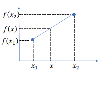
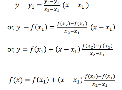
Let us find the equation of straight line from the given two points (𝑥1, 𝑓 𝑥1 ) and (𝑥2, 𝑓 𝑥2 ) .
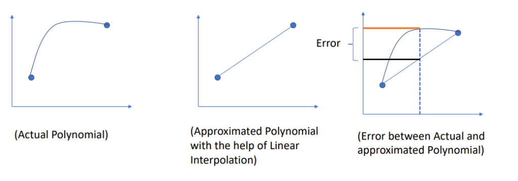
Demerits of Linear Interpolation
- Linear Interpolation uses first order polynomial (i.e. straight line) to approximate the function.
- To reduce this error, we need to use higher order polynomial.
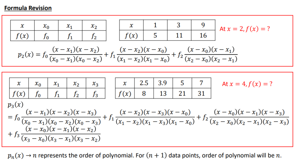
Lagrange Interpolation Polynomial
- Let 𝑥0, 𝑓0 , 𝑥1, 𝑓1 , and 𝑥2, 𝑓2 are the given data points.
| x | 𝑥0 | 𝑥1 | 𝑥2 |
| f | 𝑓0 | 𝑓1 | 𝑓2 |
Here, number of data points = 3 , so the polynomial will be of the order 2.
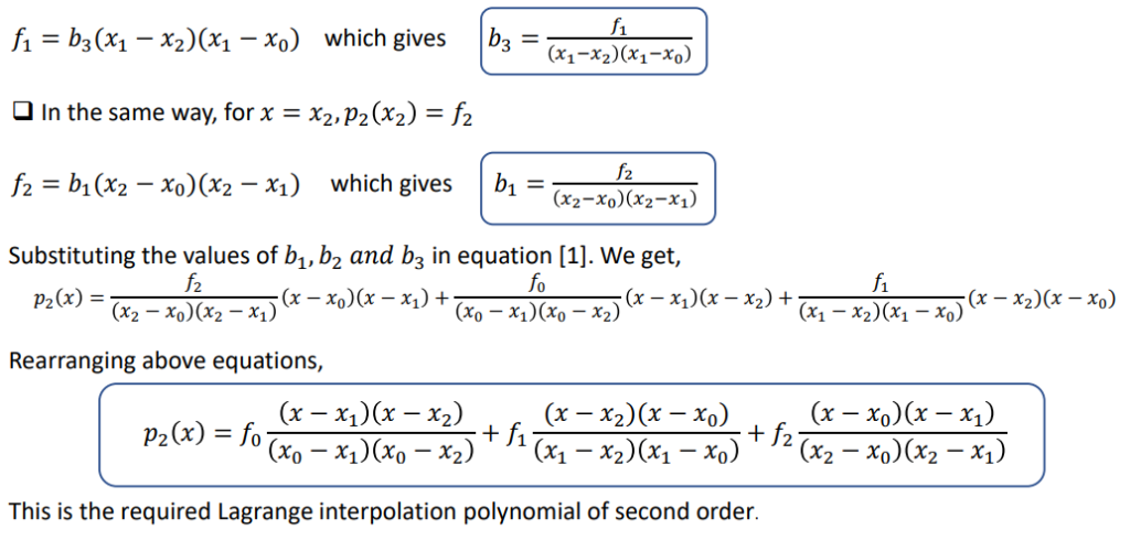
- Let us consider a second order polynomial of the form 𝑝2 𝑥 = 𝑏1 𝑥 − 𝑥0 𝑥 − 𝑥1 + 𝑏2 𝑥 − 𝑥1 𝑥 − 𝑥2 + 𝑏3 𝑥 − 𝑥2 𝑥 − 𝑥0 ………………..[1] where 𝑏1, 𝑏2 𝑎𝑛𝑑 𝑏3 𝑎𝑟𝑒 𝑡ℎ𝑒 𝑐𝑜𝑓𝑓𝑖𝑐𝑖𝑒𝑛𝑡𝑠 𝑜𝑓 𝑝𝑜𝑙𝑦𝑛𝑜𝑚𝑖𝑎𝑙.
- Given points 𝑥0, 𝑓0 , 𝑥1, 𝑓1 , and 𝑥2, 𝑓2 should satisfy the equation 1.
- At 𝑥 = 𝑥𝑜, 𝑝2 𝑥0 = 𝑓𝑜,

Similarly, for 𝑥 = 𝑥1, 𝑝2 𝑥1 = 𝑓1
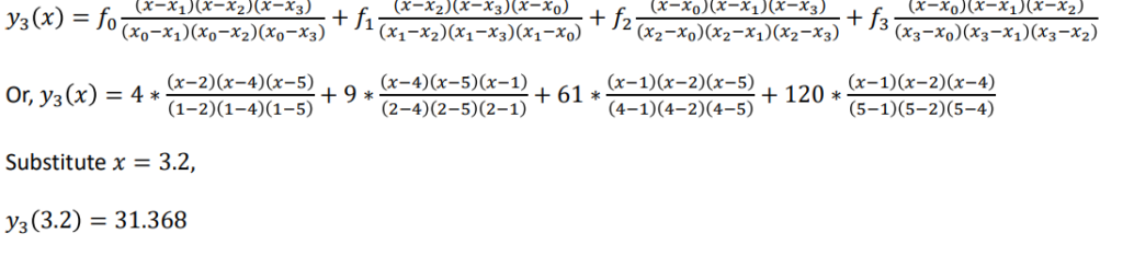
Example 2.1
For the following data ,use Lagrange interpolation polynomial to find 𝑦 𝑎𝑡 𝑥 = 3.2.
| x | 1 | 2 | 4 | 5 |
| y | 4 | 9 | 61 | 120 |
Solution: Here, 𝑥0 = 1, 𝑥1 = 2, 𝑥2 = 4, 𝑥3 = 5 , 𝑓0 = 4, 𝑓1 = 9, 𝑓2 = 61, 𝑓3 = 120
Now,
Newton Interpolation Polynomial
- The Newton form of polynomial is 𝒑𝒏 (𝒙) = 𝒂𝟎+ 𝒂𝟏𝒙 − 𝒙𝟎 + 𝒂𝟐 𝒙 − 𝒙𝟎 𝒙 − 𝒙𝟏 + 𝒂𝟑 𝒙 − 𝒙𝟎 𝒙 − 𝒙𝟏 𝒙 − 𝒙𝟐… … … … … . . +𝒂𝒏 𝒙 − 𝒙𝟎 𝒙 − 𝒙𝟏 … . . (𝒙 − 𝒙𝒏−𝟏)
- For given 𝑥0, 𝑓0 , 𝑥1, 𝑓1 , 𝑥2, 𝑓2 … … … (𝑥𝑛, 𝑓𝑛), we need to find the value of coefficients 𝑎0, 𝑎1, 𝑎2, 𝑎3 … … … . . 𝑎𝑛.
| ✓ If only two data points 𝑥0, 𝑓0 , 𝑥1, 𝑓1 are given, 𝒑𝟏 𝒙 = 𝒂𝟎+ 𝒂𝟏 𝒙 − 𝒙𝟎 → 𝟏𝒔𝒕 𝒐𝒓𝒅𝒆𝒓 𝒑𝒐𝒍𝒚𝒏𝒐𝒎𝒊𝒂𝒍 ✓ If three data points 𝑥0, 𝑓0 , 𝑥1, 𝑓1 , 𝑥2, 𝑓2 are given 𝒑𝟐 𝒙 = 𝒂𝟎 + 𝒂𝟏 𝒙 − 𝒙𝟎 + 𝒂𝟐 𝒙 − 𝒙𝟎 𝒙 − 𝒙𝟏 → 𝟐𝒏𝒅 𝒐𝒓𝒅𝒆𝒓 𝒑𝒐𝒍𝒚𝒏𝒐𝒎𝒊𝒂𝒍 ✓ Similarly, for four data points 𝑥0, 𝑓0 , 𝑥1, 𝑓1 , 𝑥2, 𝑓2 𝑥3, 𝑓3 , 𝒑𝟑 𝒙 = 𝒂𝟎 + 𝒂𝟏 𝒙 − 𝒙𝟎 + 𝒂𝟐 𝒙 − 𝒙𝟎 𝒙 − 𝒙𝟏 + 𝒂𝟑(𝒙 − 𝒙𝟎)(𝒙 − 𝒙𝟏)(𝒙 − 𝒙𝟐) → 𝟑𝒓𝒅 𝒐𝒓𝒅𝒆𝒓 𝒑𝒐𝒍𝒚𝒏𝒐𝒎𝒊𝒂𝒍 |
- For 𝑥 = 𝑥0, 𝑝𝑛 (𝑥0 )= 𝑓0 , we will get 𝑓0 = 𝑎0 . 𝑎0 = 𝑓0
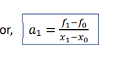
- For 𝑥 = 𝑥1, 𝑝𝑛 (𝑥1 ) = 𝑓1
or, 𝑓1 = 𝑎0 + 𝑎1 𝑥1 − 𝑥0
or, 𝑓1 = 𝑓0 + 𝑎1 𝑥1 − 𝑥0 [since 𝑎0 = 𝑓0]
𝑓2 = 𝑎0 + 𝑎1 𝑥2 − 𝑥0 + 𝑎2(𝑥2 − 𝑥0)(𝑥2 − 𝑥1) which gives

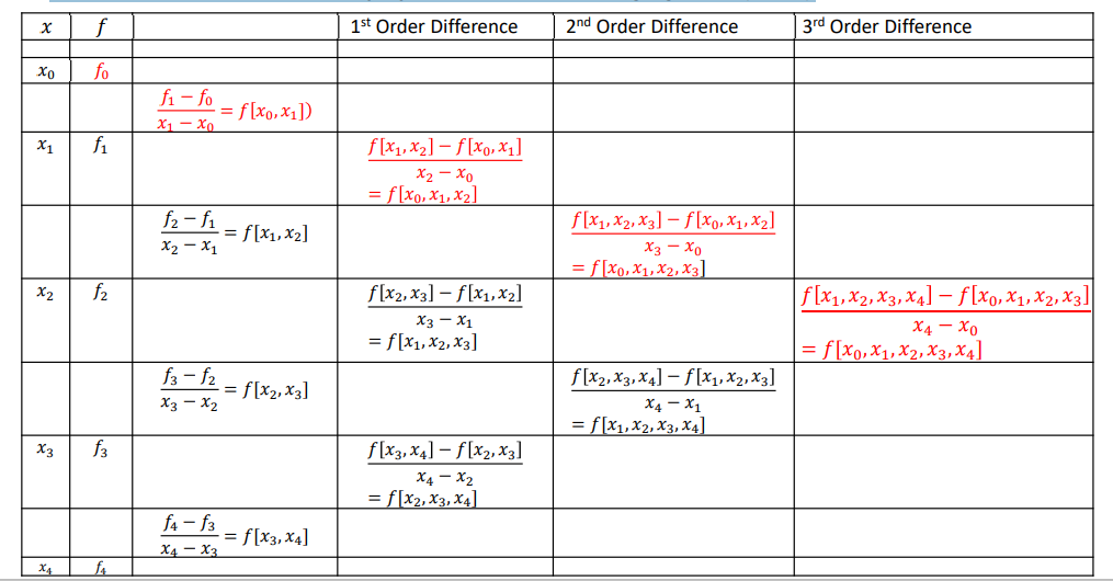
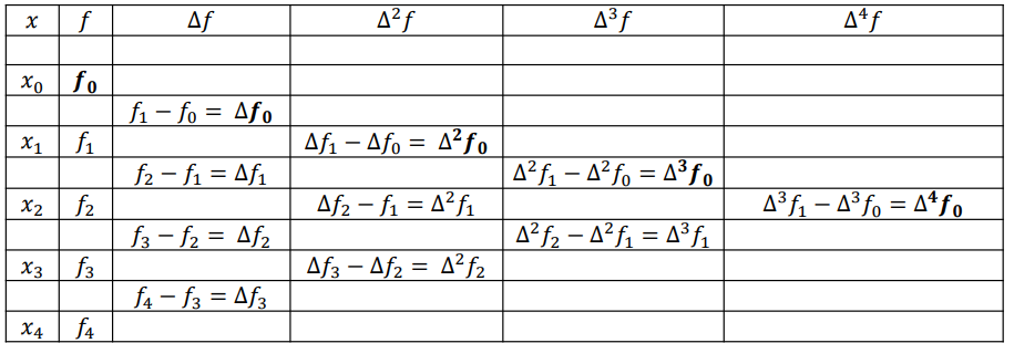
Newton Divide Difference Table
The alternative way of finding the coefficients (𝑎0, 𝑎1, 𝑎2 𝑎𝑛𝑑 𝑠𝑜 𝑜𝑛) value is to use Newton divided difference table. For given 𝑥0, 𝑓0 , 𝑥1, 𝑓1 , 𝑥2, 𝑓2 , 𝑥3, 𝑓3 𝑎𝑛𝑑 (𝑥4, 𝑓4)
Example 2.2
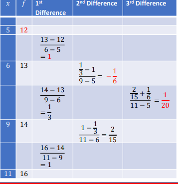
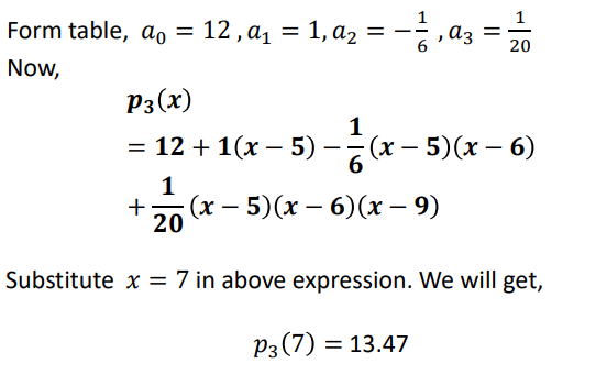
Find the functional value for 𝑥 = 7 using Newton interpolation polynomial.
| x | 5 | 6 | 9 | 11 |
| 𝑓(𝑥) | 12 | 13 | 14 | 16 |
Solution: Since 4 data points are given, the required polynomial will be of the order 3.
𝒑𝟑 (𝒙) = 𝒂𝟎 + 𝒂𝟏 𝒙 − 𝒙𝟎 + 𝒂𝟐 𝒙 − 𝒙𝟎 𝒙 − 𝒙𝟏 + 𝒂𝟑 𝒙 − 𝒙𝟎𝒙 − 𝒙𝟏 𝒙 − 𝒙𝟐
To get the value of 𝑎0, 𝑎1, 𝑎2, 𝑎3 𝑎𝑛𝑑 𝑎4 , we are going to use Newton divided difference table.
Newton Forward Difference /Newton Backward Difference [Interpolation with equidistant points]
- Particularly used when the functional values are given at a sequence of equally spaced points.
- Also called as Newton Gregory technique.
Scenario 1:
| x | 5 | 6 | 9 | 11 |
| 𝑓(𝑥) | 12 | 13 | 14 | 16 |
𝐻𝑒𝑟𝑒, 𝑥1 − 𝑥0 = 6 − 5 = 1 𝑤ℎ𝑒𝑟𝑒𝑎𝑠, 𝑥2 − 𝑥1 = 9 − 6 = 3 Not equally spaced. We can’t use Newton Forward/Backward Difference. Rather, we need to rely on Lagrange or Newton Interpolation polynomial.
Scenario 2:
| x | 10 | 20 | 30 | 40 | 50 |
| 𝑓(𝑥) | 0 | 7 | 26 | 63 | 124 |
Here, 𝒙 values are equally spaced. In this case we can use Newton forward difference or Newton backward difference.
𝑠𝑡𝑒𝑝 𝑠𝑖𝑧𝑒 ℎ = 10
- If required point is close to the start of the table, use Newton forward difference. 𝐴𝑡 𝑥 = 15, 𝑓 (𝑥) = ? 𝑜𝑟 𝐴𝑡 𝑥 = 25, 𝑓 𝑥 = ? [ First value of 𝒙 (𝐢. 𝐞. 𝑥0) acts as a reference point ]
- If required point is close to the end of the table , use Newton backward difference. 𝐴𝑡 𝑥 = 48, 𝑓 𝑥 =? 𝑜𝑟 𝐴𝑡 𝑥 = 35, 𝑥 = ? [ Last value of 𝒙 (𝐢. 𝐞. 𝑥𝑛) acts as a reference point ]
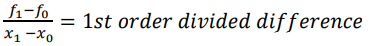
- Simple difference is used here rather than divided difference which was used in Newton divided difference table. 𝑓1 − 𝑓0 = 1𝑠𝑡 𝑜𝑟𝑑𝑒𝑟 𝑠𝑖𝑚𝑝𝑙𝑒 𝑑𝑖𝑓𝑓𝑒𝑟𝑒𝑛𝑐𝑒
Newton Forward Difference
Let us create a forward difference table for given 𝑥0, 𝑓0 , 𝑥1, 𝑓1 , 𝑥2, 𝑓2 , 𝑥3, 𝑓3 𝑎𝑛𝑑 (𝑥4, 𝑓4)
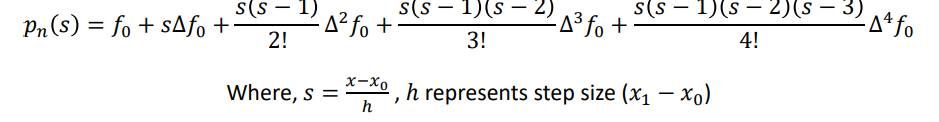
Then, the Newton forward difference formula is given by,
Example 2.3:
Estimate the value of 𝑠𝑖𝑛𝜃 𝑎𝑡 𝜃 = 250 using Newton-Gregory forward difference formula.
| 𝜃 | 10 | 20 | 30 | 40 | 50 |
| sin(𝜃) | 0.1736 | 0.3420 | 0.5000 | 0.6428 | 0.7660 |
Solution: Let us draw a Newton forward difference table to find the value of coefficients
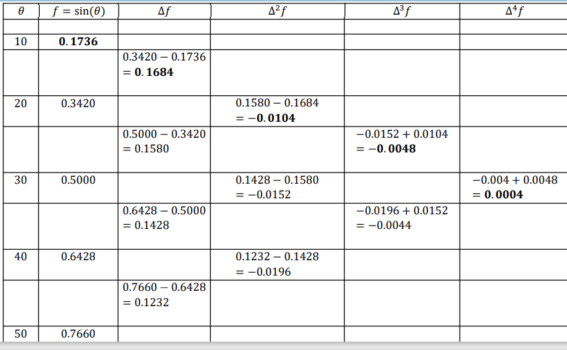
𝒇𝟎 = 𝟎. 𝟏𝟕𝟑𝟔 , ∆𝒇𝟎 = 𝟎. 𝟏𝟔𝟖𝟒, ∆ 𝟐𝒇𝟎 = −𝟎. 𝟎𝟏𝟎𝟒 , ∆ 𝟑𝒇𝟎 = −𝟎. 𝟎𝟎𝟒𝟖, ∆ 𝟒𝒇𝟎 = 𝟎. 𝟎𝟎𝟎4
Newton forward difference formula is given by,
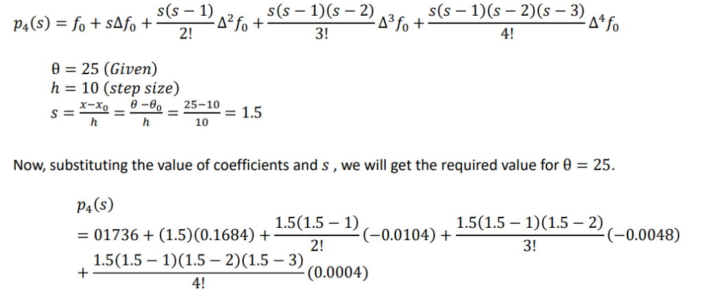
= 0.422665625
Newton Backward Difference
Let us create a forward difference table for given 𝑥0, 𝑓0 , 𝑥1, 𝑓1 , 𝑥2, 𝑓2 , 𝑥3, 𝑓3 𝑎𝑛𝑑 (𝑥4, 𝑓4)

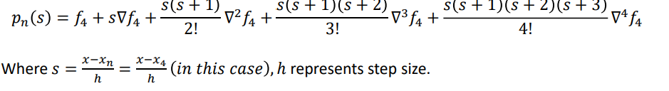
Then, the Newton backward difference formula is given by,
Example 2.4
Estimate the value of 𝑠𝑖𝑛𝜃 𝑎𝑡 𝜃 = 45 0using Newton-Gregory backward difference formula.
| 𝜃 | 10 | 20 | 30 | 40 | 50 |
| sin(𝜃) | 0.1736 | 0.3420 | 0.5000 | 0.6428 | 0.7660 |
Solution: Let us draw a Newton backward difference table to find the value of coefficients

From table, 𝑓4 = 0. 7660, 𝛻𝑓4 = 0.1232, 𝛻 2 𝑓4 = −0. 0196, 𝛻 3 𝑓4 = −0.0044, 𝑎𝑛𝑑 𝛻 4 𝑓4 = 0.0004
Newton backward difference formula is given by
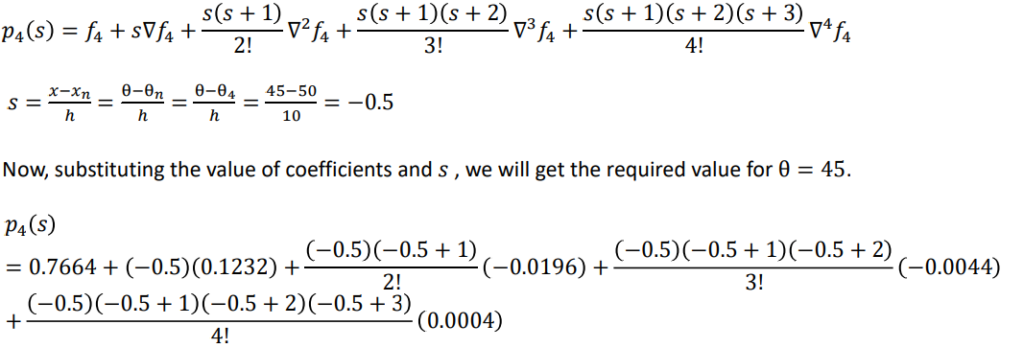
= 0.707509
NUMERICAL DIFFERENTIATION
Numerical Differentiation
- Numerical differentiation is the process of computing the value of the derivative of an explicitly unknown function, with given discrete set of points(𝑥𝑖 , 𝑓𝑖) .
- To differentiate a function numerically, we first determine an interpolating polynomial and then compute the approximate derivative at the given point.
- If 𝑥𝑖 ’s are equispaced use Newton’s forward/backward interpolation formula to find the derivative.
- If 𝑥𝑖 ’s are not equispaced, we may find using Newton’s divided difference method or Lagrange’s interpolation formula and then differentiate it as many times as required.
| Problem Scenario: The following table gives the displacement, x (cm) of an object at various of time ,t(seconds). Find the velocity and acceleration of the object at t=1.2 sec. Use suitable interpolation method. t 1.0 1.2 1.4 1.6 1.8 x 9.0 9.5 10.2 11.0 13.2 |
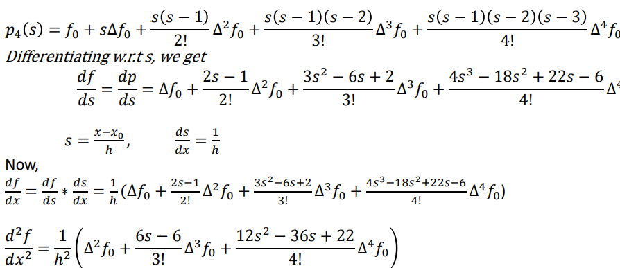
Numerical Derivatives using Newton Forward Interpolation
Newton forward interpolation formula is given by,
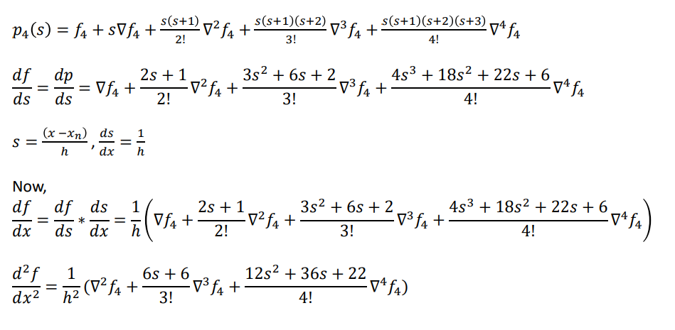
Numerical Derivatives using Newton Backward Interpolation
For given 𝑥0, 𝑓0 , 𝑥1, 𝑓1 , 𝑥2, 𝑓2 , 𝑥3, 𝑓3 𝑎𝑛𝑑 (𝑥4, 𝑓4) , Newton backward interpolation formula is given by
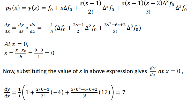
Example 2.5
| x | 0 | 1 | 2 | 3 |
| y | 5 | 6 | 3 | 8 |
Solution:
Newton difference table,
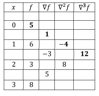
Formula for Newton forward interpolation is given by,

Example 2.6 Following table gives the census population of a state for the 1961 to 2001.
| Year | 1961 | 1971 | 1981 | 1991 | 2001 |
| Population(million) | 19.96 | 36.65 | 58.81 | 77.21 | 94.61 |
Find the rate of growth of the population in the year 2001.
Solution: since given table is equi-spaced (h=10) and rate of growth is asked for 2001, we have to
use Newton backward interpolation.
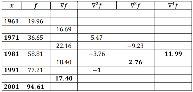
𝑓4 = 94.61, ∇ 𝑓4 = 17.40, ∇ 2 𝑓4 = −1, ∇ 3 𝑓4 = 2.76, ∇ 4 𝑓4 = 11.99
Newton Backward Interpolation formula is give by,

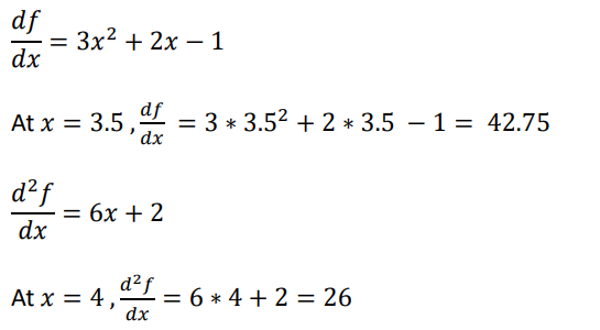
Example 2.7 Compute f ’(3.5) and f ’’(4) given that f(0)=2, f(1)=3, f(2)=12, and f(5)=147
Solution:
| x | 0 | 1 | 2 | 5 |
| y | 2 | 3 | 12 | 147 |
Since 𝑥𝑖 ′s values are not equally spaced, we have to use either Lagrange or Newton divided difference formula.
Let us draw Newton divide difference table,
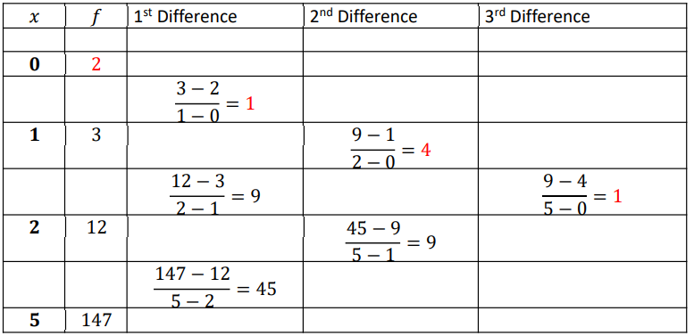
From table, 𝑎0 = 2, 𝑎1 = 1, 𝑎2 = 4, 𝑎3 = 1
Newton interpolation formula is given by,
𝑓( 𝑥) = 𝑝3( 𝑥 )= 𝑎0 + 𝑎1 𝑥 − 𝑥0 + 𝑎2 𝑥 − 𝑥0 𝑥 − 𝑥1 + 𝑎3(𝑥 − 𝑥0)(𝑥 − 𝑥1)(𝑥 − 𝑥2)
Substituting the value of coefficients,
𝑓( 𝑥) = 2 + 1 𝑥 − 0 + 4 𝑥 − 0 𝑥 − 1 + 1(𝑥 − 0)(𝑥 − 1)(𝑥 − 2)
𝑓 (𝑥) = 𝑥 3 + 𝑥 2 − 𝑥 + 2
REGRESSION

Regression : Introduction
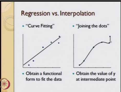
•Interpolation: If we’re provided with various scattered data points then we try to find a curve
such that all the data points will exactly pass through it.(Perfect match)
•Regression: Here we try to fit a specific form of curve to the given data points. So, it may be
possible that all the points might not pass through the curve.(Generalizes the data)
Linear Regression
Fitting straight line to the given data points.
For given data points we need only one straight line (linear) which best fits the data.
The general form of equation:
𝒚 = 𝒂 + 𝒃𝒙
Value of coefficients a, b will be calculated with the help of given data points.
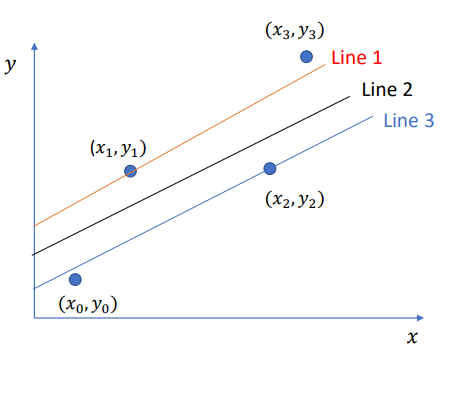
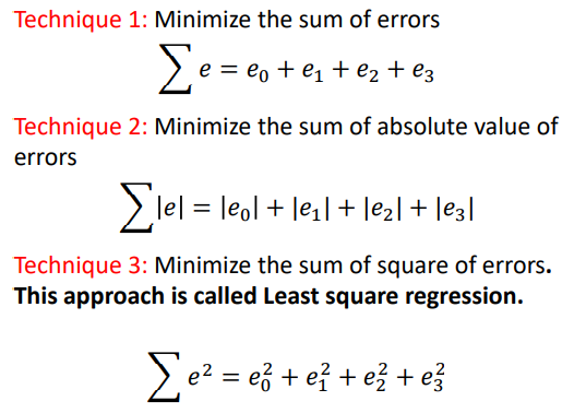
Linear Regression : Best Fitting Techniques

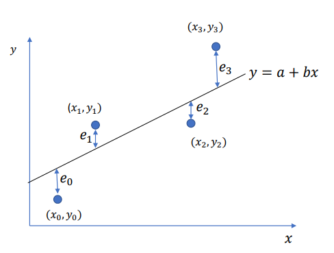
𝑒𝑟𝑟𝑜𝑟 = 𝑡𝑟𝑢𝑒 𝑣𝑎𝑙𝑢𝑒 − 𝑣𝑎𝑙𝑢𝑒 𝑜𝑏𝑡𝑎𝑖𝑛𝑒𝑑 𝑓𝑟𝑜𝑚 𝑓𝑖𝑡𝑡𝑒𝑑 𝑒𝑞𝑢𝑎𝑡𝑖𝑜𝑛
𝑒0 = 𝑦0 − (𝑎 + 𝑏𝑥0)
𝑒1 = 𝑦1 − (𝑎 + 𝑏𝑥1)
𝑒2 = 𝑦2 − (𝑎 + 𝑏𝑥2)
𝑒3 = 𝑦3 − (𝑎 + 𝑏𝑥3) 𝑦 = 𝑎 + 𝑏𝑥
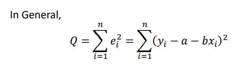
In General, 𝑒𝑖 = 𝑦𝑖 − 𝑎 + 𝑏𝑥𝑖 = 𝑦𝑖 − 𝑎 − 𝑏𝑥i
Least Square Regression
I. Fitting Linear Equation of the form 𝒚 = 𝒂 + 𝒃x
Error for each data point can be expressed as ,
𝑒𝑖 = 𝑦𝑖 − 𝑎 + 𝑏𝑥𝑖 = 𝑦𝑖 − 𝑎 – 𝑏𝑥𝑖
In least squared approach, we use sum of square of errors, i.e
Total Error 𝑄 = 𝑒1 2 + 𝑒2 2 + 𝑒3 2 + 𝑒4 2 + … … … . . +𝑒𝑛 2
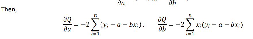
We have to choose 𝑎 𝑎𝑛𝑑 𝑏 such that total error 𝑄 is minimum. Since 𝑄 depends on 𝑎 𝑎𝑛𝑑 𝑏 , a necessary
condition for 𝑄 to be minimum is,

Example 2.8 Fit a straight line for the following data
| x | 1 | 2 | 3 | 4 | 5 |
| y | 3 | 4 | 5 | 6 | 8 |
Solution:
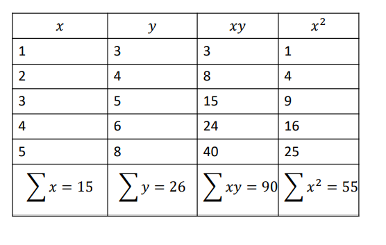
We have to fit straight line of the form
𝑦 = 𝑎 + 𝑏𝑥
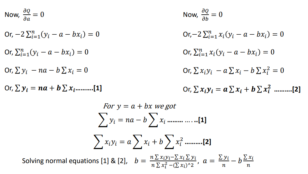
Normal equations for the above equation is,
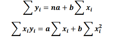
n = 5 (number of data points given in table)
Now,
26 = 5𝑎 + 15𝑏
90 = 15𝑎 + 55𝑏
Upon solving these two equations, we get
𝑎 = 1.60, 𝑏 = 1.20
Hence, the required straight line is, 𝑦 = 𝑎 + 𝑏𝑥 = 𝟏. 𝟔 + 𝟏. 𝟐x
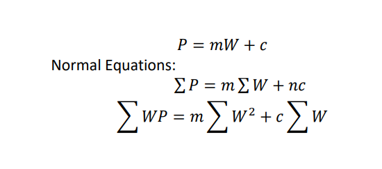
Example 2.9: If P is pull required to lift a load W by means of a pulley, find a linear law of the form 𝑃 =
𝑚𝑊 + 𝑐 using the following data. Also, find the value of P for W =30.
P 12 15 21 25
W 50 70 100 120
Hint: In 𝑃 = 𝑚𝑊 + 𝑐, 𝑚 𝑎𝑛𝑑 𝑐 are the coefficients whose value is to be determined with the help of given
data.


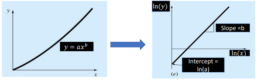
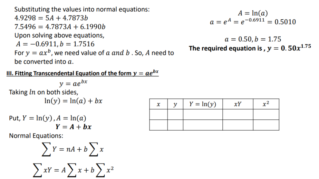
II. Fitting Power Equation of the form 𝒚 = 𝒂𝒃 𝒙
The power equation 𝑦 = 𝑎𝑏 𝑥 is non linear in the form. First of all, we need to represent it into linear form.
𝑦 = 𝑎𝑥 𝑏
Taking 𝑙𝑛 on both sides,
ln 𝑦 = ln(𝑎𝑥 𝑏 )
ln 𝑦 = ln 𝑎 + 𝑏 ln(𝑥)
Let us suppose, 𝑌 = ln 𝑦 , 𝐴 = ln 𝐴 , 𝑋 = ln 𝑥 . We get, 𝑌 = 𝐴 + 𝑏 𝑋 (Linear Form )

References :
- Balagurusamy, E. Numerical Methods. New Delhi: Tata McGraw-Hill Publishing Company Limited, 2008.
- Sastry, S.S. Introductory Methods of Numerical Analysis. New Delhi: PHI Learning Pvt. Ltd., 2012.
- Steven C. Chopra, Raymond P. Canale. Numerical Methods for Engineers. Newyork: MCGraw Hill Education,
2015.