
CORRELATION
In many natural systems, changes in one attribute are accompanied by changes in another attribute and that a definite relation exists between the two. In other words, there is a correlation between the two variables. For instance, several soil properties like nitrogen content, organic carbon content or pH are correlated and exhibit simultaneous variation. Strong correlation is found to occur between several morphometric features of a tree. In such instances, an investigator may be interested in measuring the strength of the relationship. Having made a set of paired observations (xi,yi); i = 1, …, n, from n, independent sampling units, a measure of the linear relationship between two variables can be obtained by the following quantity called Pearson’s product moment correlation coefficient or simply correlation coefficient.
Definition: If the change in one variable affects a change in the other variable, the two variables are said to be correlated and the degree of association ship (or extent of the relationship) is known as correlation.
Types of correlation:
a). Positive correlation: If the two variables deviate in the same direction, i.e., if the increase (or decrease) in one variable results in a corresponding increase (or decrease) in the other variable, correlation is said to be direct or positive.
Ex: (i) Heights and weights
(ii) Household income and expenditure
(iii) Amount of rainfall and yield of crops
(iv) Prices and supply of commodities
(v) Feed and milk yield of an animal
(vi) Soluble nitrogen and total chlorophyll in the leaves of paddy.
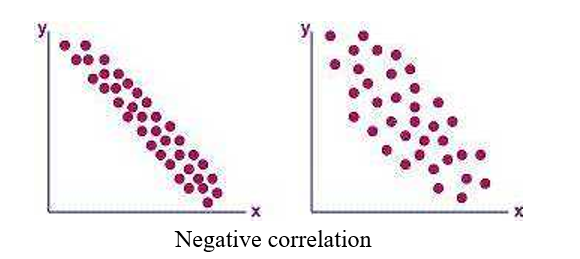
b) Negative correlation: If the two variables constantly deviate in the opposite direction i.e., if increase (or decrease) in one variable results in corresponding decrease (or increase) in the other variable, correlation is said to be inverse or negative.
Ex: (i) Price and demand of a goods
(ii) Volume and pressure of perfect gas
(iii) Sales of woolen garments and the day temperature
(iv) Yield of crop and plant infestation
c) No or Zero Correlation: If there is no relationship between the two variables such that the value of one variable change and the other variable remain constant is called no or zero correlation.
Methods of studying correlation:
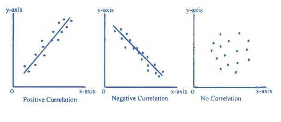
1. Scatter Diagram
2. Karl Pearson‟s Coefficient of Correlation
3. Spearman‟s Rank Correlation
4. Regression Lines
1. Scatter Diagram
It is the simplest way of the diagrammatic representation of bivariate data. Thus for the bivariate distribution (xi,yi); i = j = 1,2,…n, If the values of the variables X and Y be plotted along the X-axis and Y-axis respectively in the xy-plane, the diagram of dots so obtained is known as scatter diagram. From the scatter diagram, if the points are very close to each other, we should expect a fairly good amount of correlation between the variables and if the points are widely scattered, a poor correlation is expected. This method, however, is not suitable if the number of observations is fairly large.
If the plotted points show an upward trend of a straight line, then we say that both the variables are positively correlated.

When the plotted points shows a downward trend of a straight line then we say that both the variables are negatively correlated.
If the plotted points spread on whole of the graph sheet, then we say that both the variables are not correlated.

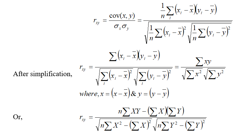
2. Karl Pearson‟s Coefficient of Correlation
Prof. Karl Pearson, a British Biometrician suggested a measure of correlation between two variables. It is known as Karl Pearson‟s coefficient of correlation. It is useful for measuring the degree and direction of linear relationship between the two variables X and Y. It is usually denoted by rxy or r(x,y) or ‘r’.
a. Direct method
b. When deviations are taken from an assumed mean.
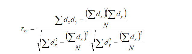
Where,
n = number of items; dx = x-A, dy = y-B
A = assumed value of x and B = assumed value of y
c. By changing origin
mean value of Y series.
If U = X-A and V = Y-B
Where, A= Assumed mean value of X series.
B = Assumed

d. By changing origin and scale.
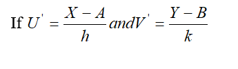
Where, A = Assumed mean in value of X series
B = Assumed mean in value of Y series.
h = common factor or width of class interval of X series.
k = Common factor or width of class interval of Y series.

- The correlation coefficient never exceeds unity. It always lies between –1 and +1. (i.e. –1≤ r ≤1)
- If r = +1 then we say that there is a perfect positive correlation between x and y.
- If r = -1 then we say that there is a perfect negative correlation between x and y .
- If r = 0 then the two variables x and y are called uncorrelated variables.
- Correlation coefficient (r) is the geometric mean between two regression coefficients. i.e. , where bxy and byx are regression coefficient of X on Y and Y on X respectively.
- Correlation coefficient is independent of change of origin and scale.
| Interpretation of correlation coefficient If the correlation coefficient lies between, ±1 , : Then correlation is perfect. ±0.75 to ±1 : Then correlation is very high (significant). ±0.50 to ±0.75 : Then the correlation is high. ±0.25 to ±0.50 : Then the correlation is low. 0 to ± 0.25, : Then the correlation is very low (insignificant) 0, : No correlation. |
Test for significance of correlation coefficient
If “r” is the observed correlation coefficient in a sample of ‘n’ pairs of observations from a bivariate normal population, then Prof. Fisher proved that under the null hypothesis
H0 : r = 0
the variables x, y follows a bivariate normal distribution. If the population correlation coefficient of x and y is denoted by ρ, then it is often of interest to test whether ρ is zero or different from zero, on the basis of observed correlation coefficient “r”. Thus if “r” is the sample correlation coefficient based on a sample of
“n” observations, then the appropriate test statistic for testing the null hypothesis
H0 : r = 0 against the alternative hypothesis H1: r ≠ 0 is
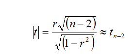
“t” follows Student’s t – distribution with (n-2) d.f.
If calculated value of |t| > is greater than critical value of t (n-2) d.f. at specified level of significance, then the null hypothesis is rejected. That is, there may be significant coefficient correlation between two variables. Otherwise, the null hypothesis is accepted.
Example: Consider the data on pH and organic carbon content measured from soil
samples collected from 12 pits taken in natural forests, given in table.
Table : Values of pH and organic carbon content observed in soil samples
collected from natural forest.
| Soil pit | 1 | 2 | 3 | 4 | 5 | 6 | 7 | 8 | 9 | 10 | 11 | 12 |
| pH(x) | 5.7 | 6.1 | 5.2 | 5.7 | 5.6 | 5.1 | 5.8 | 5.5 | 5.4 | 5.9 | 5.3 | 5.4 |
| Organic carbon(%) (y) | 2.10 | 2.17 | 1.97 | 1.39 | 2.26 | 1.29 | 1.17 | 1.14 | 2.09 | 1.01 | 0.89 | 1.60 |
Find the correlation coefficient between values of pH and organic carbon content. Also test the significance of observed correlation coefficient at 5% level of significance.
Solution:
Direct method;
Calculation of correlation
| Soil pit | pH(x) | Organic carbon (%) (y) | (x2) | (y2) | (x y) |
| 1 | 5.7 | 2.1 | 32.49 | 4.41 | 11.97 |
| 2 | 6.1 | 2.17 | 37.21 | 4.7089 | 13.24 |
| 3 | 5.2 | 1.97 | 27.04 | 3.8809 | 10.24 |
| 4 | 5.7 | 1.39 | 32.49 | 1.9321 | 7.92 |
| 5 | 5.6 | 2.26 | 31.36 | 5.1076 | 12.66 |
| 6 | 5.1 | 1.29 | 26.01 | 1.6641 | 6.58 |
| 7 | 5.8 | 1.17 | 33.64 | 1.3689 | 6.79 |
| 8 | 5.5 | 1.14 | 30.25 | 1.2996 | 6.27 |
| 9 | 5.4 | 2.09 | 29.16 | 4.3681 | 11.29 |
| 10 | 5.9 | 1.01 | 34.81 | 1.0201 | 5.96 |
| 11 | 5.3 | 0.89 | 28.09 | 0.7921 | 4.72 |
| 12 | 5.4 | 1.6 | 29.16 | 2.56 | 8.64 |
| Total | 66.7 | 19.08 | 371.71 | 33.1124 | 106.28 |
Then, correlation coefficient is,
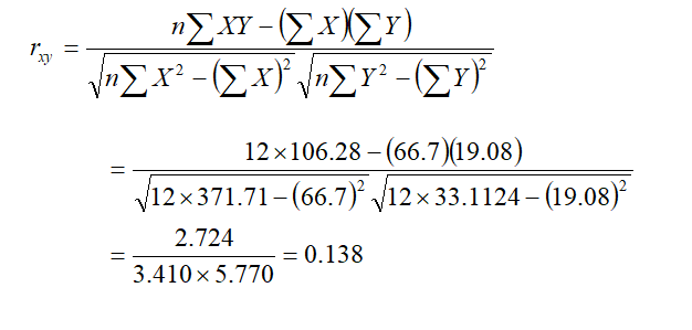
Here, r = 0.138, which means there is positive and very low correlation or insignificant correlation between ph and organic carbon content.
Test of significance of observed correlation coefficient.
Null hypothesis, H0: r = 0
Alternative hypothesis, H1: r ≠0
Under null hypothesis test statistic is ;

The critical value of t is 2.23, for 10 degrees of freedom at the probability level, a = 0.05. Since the computed t value is less than the critical value, we conclude that the pH and organic carbon content measured from soil samples are not significantly correlated.
Rank correlation
Before learning about Spearman’s correlation it is important to understand Pearson’s correlation which is a statistical measure of the strength of a linear relationship between paired data. Its calculation and subsequent significance testing of it requires the following data assumptions to hold:
· interval or ratio level;
· linearly related;
· bivariate normally distributed.
If your data does not meet the above assumptions, then use Spearman’s rank correlation.
Monotonic function
To understand Spearman’s correlation, it is necessary to know what a monotonic function is. A monotonic function is one that either never increases or never decreases as its independent variable increases. The following graphs illustrate monotonic function.
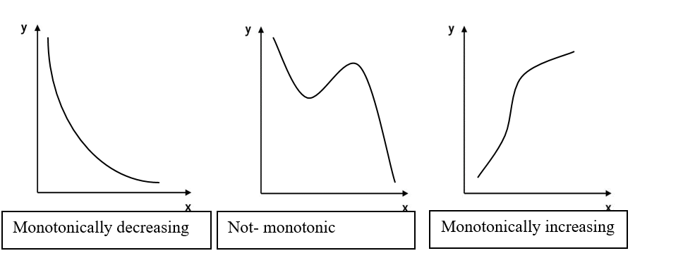
· Monotonically increasing – as the ‘x’ variable increases the ‘y’ variable never decreases;
· Monotonically decreasing – as the ‘x’ variable increases the ‘y’ variable never increases;
· Not monotonic – as the ‘x’ variable increases the ‘y’ variable sometimes decreases and sometimes increases.
3. Spearman’s rank correlation:
When the data is non- normal or qualitative, e.g., intelligence, beauty, honesty, taste etc. Karl Pearson’s coefficient of correlation cannot be used. In such cases we arrange the variables or individuals in order of merit and proficiency and assign ranks. The coefficient of rank correlation as given by Spearman is
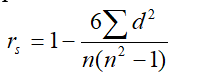
Where, rs = Spearman’s rank correlation coefficient
d = difference of corresponding ranks (i.e., d = xi-yi or d = Rx-Ry )
Note:
If ranks are repeated or tied then above formula of Spearman’s rank correlation coefficient become,
Where denotes the number of times an item is repeated.
Example :
Calculate the rank correlation coefficient from the following data.
| X | 80 | 78 | 75 | 75 | 68 | 67 | 68 | 59 |
| Y | 12 | 13 | 14 | 14 | 14 | 16 | 15 | 17 |
Solution:
Let Rx be the rank of X series and Ry be the rank of Y series.
Calculation of Rank correlation coefficient
| X | Y | Rx | Ry | d = Rx –Ry | d2 |
| 80 | 12 | 1 | 8 | -7 | 49 |
| 78 | 13 | 2 | 7 | -5 | 25 |
| 75 | 14 | 3.5 | 5 | -1.5 | 2.25 |
| 75 | 14 | 3.5 | 5 | -1.5 | 2.25 |
| 68 | 14 | 5.5 | 5 | 0.5 | 0.25 |
| 67 | 16 | 7 | 2 | 5 | 25 |
| 68 | 15 | 5.5 | 3 | 2.5 | 6.25 |
| 59 | 17 | 8 | 1 | 7 | 49 |
| Total | 159 |
Here, in X series two items 75 and 68 repeated 2-times each.
So, m1 = 2, m2 = 2
Again in Y series one item 14 is repeated 3 times.
So, m3 = 3 Thus rank correlation coefficient is ;


Here rs = – 0.93, which shows that there is very high but negative relationship between two variables X and Y.
REGRESSION
Correlation coefficient measures the extent of interrelation between two variables which are simultaneously changing with mutually extended effects. In certain cases, changes in one variable are brought about by changes in a related variable but there need not be any mutual dependence. In other words, one variable is considered to be dependent on the other variable changes, in which are governed by extraneous factors. Relationship between variables of this kind is known as regression. When such relationships are expressed mathematically, it will enable us to predict the value of one variable from the knowledge of the other. For instance, the photosynthetic and transpiration rates of trees are found to depend on atmospheric conditions like
temperature or humidity but it is unusual to expect a reverse relationship. However, in many cases, it so happens that the declaration of certain variables as independent is made only in a statistical sense although when reverse effects are conceivable in such cases. For instance, in a volume prediction equation, tree volume is taken to be dependent on dbh although the dbh cannot be considered as independent of the effects of tree volume in a physical sense. For this reason, independent variables in the context of regression are sometimes referred as regressor or preditor or explanatory variables and the dependent variable is called the regressand or explained variable.
The dependent variable is usually denoted by y and the independent variable by x.When only two variables are involved in regression, the functional relationship is known as simple regression. If the relationship between the two variables is linear, it is known as simple linear regression, otherwise it is known as nonlinear regression. When one variable is dependent on two or more independent variables, the functional relationship between the dependent and the set of independent variables is known as multiple regression.
Simple linear regression
The simple linear regression of y on x in the population is expressible as
y = a + bx + e
Where y = dependent variable
x = independent variable
α = y- intercept (expected value of y when x assumes the value zero)
β = regression coefficient of y on x or slope of the line. (it measures the average change in the value of Y when unit change in the value of X)
ɛ = residual or error.
The slope of a linear regression line may be positive, negative or zero depending on the relation between y and x. In practical applications, the values of a and b are to be estimated from observations made on y and x variables from a sample. For instance, to estimate the parameters of a regression equation proposed between atmospheric temperature and transpiration rate of trees, a number of paired observations are made on transpiration rate and temperature at different times of the day from a number of trees. Let such pairs of values be designated as (xi, yi); i = 1, 2, . . ., n where n is the number of independent pairs of observations. The values of a and b are estimated using the method of least squares such that the sum of squares of the difference between the observed and expected value is minimum. In the estimation process, the following assumptions are made viz., (i) The x values are non-random or fixed (ii) For any given x, the variance of y is the same (iii) The y values observed at different values of x are completely independent. Appropriate changes will need to be made in the analysis when some of these assumptions are not met by the data. For the purpose of testing hypothesis of parameters, an additional assumption of normality of errors will be required.
Estimating the values of a and b using least square method.
- Regression equation of Y on X.
It is the line which gives the best estimates for the values of Y for any specified values of X.
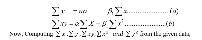
The regression equation of Y on X is given as
Y = α +βX ………………(1)
The values of two constants α and β can be determined by solving following two normal equations (applying principle of least square)
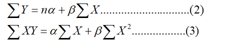
Now, substituting the value of α and β in equation (1), we get the required estimated regression equation of Y on X as,

Alternative method of estimating a and b.
Let y = a + bx + e be the simple linear regression equation of y on x
Then a and b are estimated directly as,

Testing the significance of the regression coefficient
Once the regression function parameters have been estimated, the next step in
regression analysis is to test the statistical significance of the regression function. It is
usual to set the null hypothesis against the alternative hypothesis, H1 : b ¹
0 or (H1 : b < 0 or H1 : b > 0, depending on the anticipated nature of relation). For the
testing, we may use the analysis of variance procedure.
Testing procedure:
- Set up hypothesis as;
Null hypothesis, H0: b = 0
Alternative hypothesis, H1: b ¹ 0 or (H1: b < 0 or H1: b > 0, depending on the anticipated nature of relation)
- Construct an outline of analysis of variance table as follows.
| Source of Variation (SV) | Degree of freedom (d.f.) | Sum of square (SS) | Mean sum of square (MSS=SS/d.f.) | F-ratio |
| Due to regression Error | 1 n-2 | SSR SSE | MSR MSE | MSR/MSE |
| Total | n-1 | TSS |
- Compute the different sums of squares as follows
a. Total sum of square

b. Sum of square due to regression

c. Sum of squares due to deviation from regression

- Enter the values of sums of squares in the analysis of variance table and perform the rest of the calculations.
- Compare the computed value of F with tabular value at (1,n-2) degrees of freedom. If the calculated value is greater than the tabular value of F at (1,n-2) degrees of freedom at α% level of significance then F value is significant otherwise insignificance. If the computed F value is significant, then we can state that the regression coefficient, b is significantly different from 0.
Coefficient of determination:
The coefficient of determination (r2) is a measure of the variation of the dependent variable that is explained by the regression line and the independent variable. It is often used as a measure of the correctness of a model, that is, how well a regression model will fit the data. A ‘good’ model is a model where the regression sum of squares is close to the total sum of squares, SSR ≈ TSS . A “bad” model is a model where the residual sum of squares is close to the total sum of squares, SSE ≈ TSS . The coefficient of determination represents the proportion of the total variability explained by the model.
i.e.,
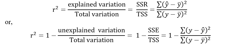
Here,
Total sum of square = Regression sum of square +Error sum of square
TSS = RSS + ESS
Of course, it is usually easier to find the coefficient of determination by squaring correlation coefficient (r) and converting it to a percentage. Therefore, if r = 0.90, then r 2 = 0.81, which is equivalentto 81%. This result means that 81% of the variation in the dependent variable isaccounted for by the variations in the independent variable. The rest of the variation,0.19, or 19%, is unexplained. This value is called the coefficient of non-determination andis found by subtracting the coefficient of determination from 1. As the value of r approaches 0, r2 decreases more rapidly. For example, if r = 0.6, then r 2 = 0.36, whichmeans that only 36% of the variation in the dependent variable can be attributed to thevariation in the independent variable. Another way to arrive at the value for r2 is to square the correlation coefficient.
The coefficient of determination can have values 0 ≤ r2 ≤ 1. The “good” model means that r2 is close to one.
Standard error of the estimate:
The standard error of estimate is the measure of variation of an observation made around the estimated regression line. Simply, it is used to check the accuracy of predictions made with the regression line.
Like, a standard deviation which measures the variation in the set of data from its mean, the standard error of estimate measures the variation in the actual values of Y from the estimated values of Y (predicted) on the regression line. The smaller the value of a standard error of estimate the closer are the dots to the regression line and better is the estimate based on the equation of the line. If the standard error is zero, then there is no variation corresponding to the computed line and the correlation will be perfect.
The standard error of estimate of ‘Y’ for given ‘X’ (i.e. Y on X) is denoted by Syx or Se and given by;
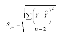
Where; Y= value of dependent variable.
= estimated value of Y.
n = number of observations in the sample.
Here, we use (n-2) instead of ‘n’ because of the fact that two degree of freedom are lost in estimating the regression line as the value of two parameters ‘β0’ and ‘β1’ are to be determined from the data.
Above formula is not convenient as it requires to calculate the estimated value of Y i.e. Thus, more convenient and easy formula is given below:
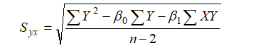
Where;
X and Y are independent and dependent variables respectively.
β0 = Y- intercept.
β1 = slope of the line.
n = number of observations in the sample.
Properties of regression lines and coefficients:
- Two regression lines pass through the mean point .
- Two regression lines coincide when the variables X and Y are perfectly correlated.
i.e. (r = ±1).
- The two regression lines are right angle to each other if X and Y are independent to each other. (i.e. when r = 0)
- The two regression lines must have same sign. Also, the correlation coefficient and regression coefficients must have the same sign.
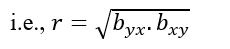
- Correlation coefficient is the geometric means between the two regression coefficients.
- The product of two regression coefficients must be less than or equal to 1.

- Regression coefficient is independent of change of origin but not scale.
Example:
The following observations are from a morphometric study of cottonwood trees. The widths of 12 leaves from a single tree were measured (in mm) while fresh and after drying.
| Fresh leaf width (X) | 90 | 115 | 55 | 110 | 76 | 100 | 84 | 95 | 84 | 95 | 100 | 90 |
| Dry leaf width (Y) | 88 | 109 | 52 | 105 | 71 | 95 | 78 | 90 | 77 | 91 | 96 | 86 |
- Estimate the parameters of simple linear regression using least square method and using the model predict the dry leaf width on the basis of 95 mm fresh leaf width.
- Find the linear relationship between fresh leaf and dry leaf width.
- Calculate the coefficient of determination and interpret it in practical manner.
- Find the standard error (Se) of the estimate.
- Test the significance of regression coefficient (β) at 5% level of significance.
Solution:
- Let y= α+ β1 x be the simple linear regression equation of Y on X.
Then its normal equations are;
| Fresh leaf (x) | Dry leaf width (y) | x2 | y2 | xy |
| 90 | 88 | 8100 | 7744 | 7920 |
| 115 | 109 | 13225 | 11881 | 12535 |
| 55 | 52 | 3025 | 2704 | 2860 |
| 110 | 105 | 12100 | 11025 | 11550 |
| 76 | 71 | 5776 | 5041 | 5396 |
| 100 | 95 | 10000 | 9025 | 9500 |
| 84 | 78 | 7056 | 6084 | 6552 |
| 95 | 90 | 9025 | 8100 | 8550 |
| 100 | 77 | 10000 | 5929 | 7700 |
| 95 | 91 | 9025 | 8281 | 8645 |
| 100 | 96 | 10000 | 9216 | 9600 |
| 90 | 86 | 8100 | 7396 | 7740 |
| 1110 | 1038 | 105432 | 92426 | 98548 |

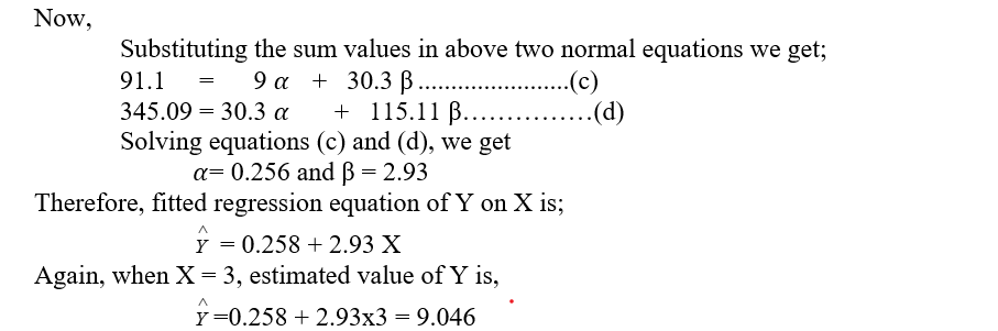
Substituting the sum values in above two normal equations we get;
1038 = 12α +1110 β ………………………..(c)
98548=1110α + 105432 β …………………..(d)
Solving equations (c) and (d), we get
α = 1.515 β = 0.919
Therefore fitted regression equation of Y on X is;
Y= 1.515 + 0.919 X …………………..(e)
Thus estimated width of dry leaf having 95 mm fresh leaf is ,
Y = 1.515+ 0.919 x 95 = 88.82 mm
- Correlation coefficient between dry and fresh leaf is ;
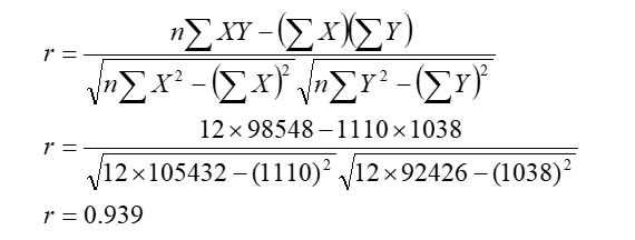
Here r = 0.929, which means there is positive and very high correlation between width of dry leaf and fresh leaf.
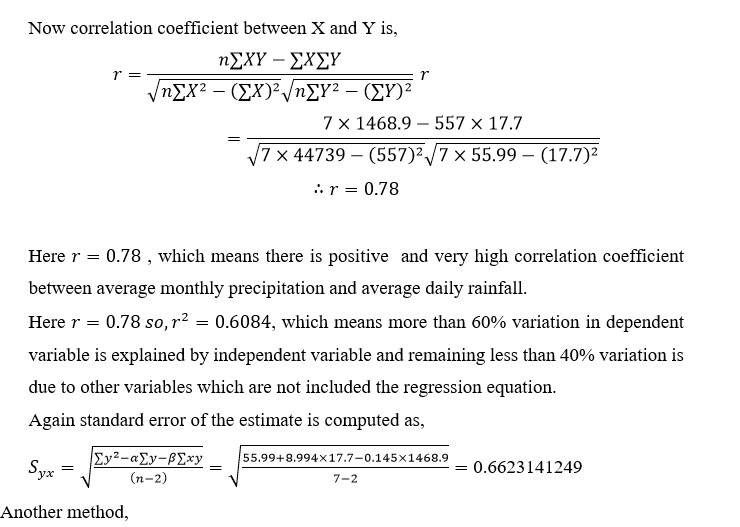
- Here r = 0.939 so r2 = 0.88, which means about 88% variation in width of dry leaf is due to fresh leaf and remaining 12 % variation is due to other variables.
- Standard error of the estimate of Y on X is,

- Test of significance of observed regression coefficient (β):
Null hypothesis (H0): β = 0
Alternative hypothesis (H1): β ≠ 0
Computing the different sums of squares as follows.
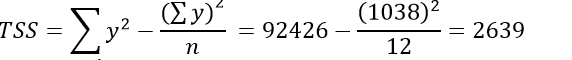
Total sum of square(TSS)
Sum of square due to regression

Sum of squares due to deviation from regression

TABLE
| Source of Variation (SV) | Degree of freedom (d.f.) | Sum of square (SS) | Mean sum of square (MSS=SS/d.f.) | F-ratio |
| Due to regression Error | 1 12-2=10 | SSR=2327.199 SSE=311.801 | MSR=2327.199 MSE= 31.1801 | = 74.637 |
| Total | n-1=11 | TSS= 2639 |
Thus test statistics F= 74.637.
Critical value of F at α= 5% level of significance for (1,10) degree of freedom is 4.96.
Decision: Here calculated value of F (74.637) is greater than critical value of F at 5% level of significance for (1,10) degree of freedom. So accept alternative hypothesis and reject null hypothesis and conclude that regression coefficient (β) is significant.
Example:1
A physical measurement, such as intensity of light of a particular wavelength transmitted through a solution, can often be calibrated to give the concentration of particular substance in the solution. ‘9’ pairs of values of intensity (X) and concentration ‘Y’ were obtained and can be summarized as follows:

- Find the regression equation of Y on X and estimate the value of Y when X=3.
- Find the coefficient of determination and interpret it.
- Compute the standard error of the estimate.
Solution:
(b) Since, square of correlation coefficient is coefficient of determination. So let us find correlation coefficient between X and Y as,
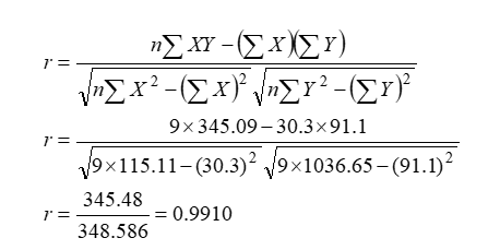
Coefficient of determination (r2) = (0.9910)2 =0.982
This gives, more than 98% of the variation in Y has able to explain by fitted regression model.
(c) Standard error of the estimate of Y on X is,

Example:2
In a study between the amount of rainfall and the quantity of air pollution removed the following data were collected:
Daily rainfall: 4.3 4.5 5.9 5.6 6.1 5.2 3.8 2.1
(in .01 cm)
Pollution removed: 12.6 12.1 11.6 11.8 11.4 11.8 13.2 14.1
(mg/m3)
Find the regression line of y on x.
Solution:
Let Y= β0 + β1X , be the simple linear regression equation of Y( Pollution removed) on X (daily rainfall).
Then its normal equations are;

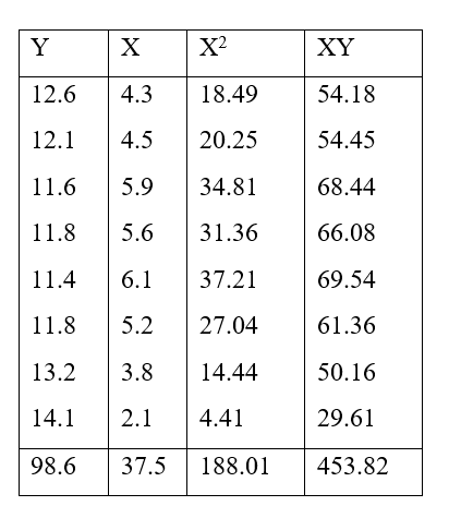
Now,
Substituting the sum values in above two normal equations we get;
98.6 = 8 β0 + 37.5 β1 …………………..(c)
453.82 = 37.5 β0 + 188.01 β1……………(d)
Solving equations (c) and (d), we get
β0= 15.532 and β1 = -0.684
Then, fitted or estimated regression line of Y on X is,

Example:
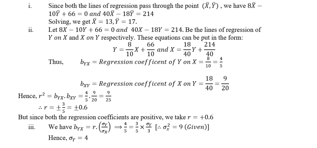
In a partially destroyed laboratory record of an analysis of correlation data, the following results only are legible:
Variable of X = 9

What were, i. The mean values of X and Y.
ii. The correlation coefficient between X and Y, and
iii. The standard deviation of Y?
Solution:
Example:
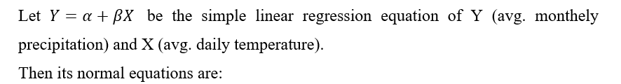
Average Temperature and Precipitation Temperatures (in degrees Fahrenheit) and precipitation (in inches) are as follows:
| Avg. daily temp. x | 86 | 81 | 83 | 89 | 80 | 74 | 64 |
| Avg. monthly precip. y | 3.4 | 1.8 | 3.5 | 3.6 | 3.7 | 1.5 | 0.2 |
- Find y when x =70F.
- Find the correlation coefficient and interpret it in practical manner.
- Find the coefficient of determination and interpret it.
- Find the standard error of the estimate.
Solution:
| Avg. daily temp. x | Avg. monthly precip. y | |||
| 86 | 3.4 | 7396 | 11.56 | 292.4 |
| 81 | 1.8 | 6561 | 3.24 | 145.8 |
| 83 | 3.5 | 6889 | 12.25 | 290.5 |
| 89 | 3.6 | 7921 | 12.96 | 320.4 |
| 80 | 3.7 | 6400 | 13.69 | 296 |
| 74 | 1.5 | 5476 | 2.25 | 111 |
| 64 | 0.2 | 4096 | 0.04 | 12.8 |
| 557 | 17.7 | 44739 | 55.99 | 1468.9 |
Now substituting the values of various sum and solving it we get,Now substituting the values of various sum and solving it we get,
Now correlation coefficient between X and Y is,
| x | y | |||
| 86 | 3.4 | 3.476 | -0.076 | 0.005776 |
| 81 | 1.8 | 2.751 | -0.951 | 0.904401 |
| 83 | 3.5 | 3.041 | 0.459 | 0.210681 |
| 89 | 3.6 | 3.911 | -0.311 | 0.096721 |
| 80 | 3.7 | 2.606 | 1.094 | 1.196836 |
| 74 | 1.5 | 1.736 | -0.236 | 0.055696 |
| 64 | 0.2 | 0.286 | -0.086 | 0.007396 |
| 557 | 17.7 | 71.771 | -54.071 | 2.477507 |

Reference : Probability and statistics for engineers by Toya Naryan Paudel & Pradeep Kunwar, Sukunda Pustak Bhawan.