

Introduction
Let us consider a set of values (𝑥𝑖, 𝑦𝑖) of a function. The process of computing the derivative or
derivatives of that function at some values of x from the given set of values is called Numerical
Differentiation. This may be done by first approximating the function by suitable interpolation
formula and then differentiating.
Derivatives using Newton’s Forward Difference formula
Newton’s forward interpolation formula
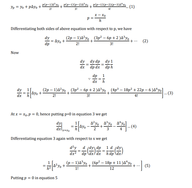

Derivate using Newton’s Backward Difference Formula
Newton’s backward interpolation formula is
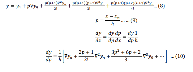
At 𝑥 = 𝑥𝑛, 𝑝 = 0, hence putting p=0 in equation 10 we get


Note: first derive is also as rate of change, so it can also be asked to find the velocity, second
derivate to find acceleration.
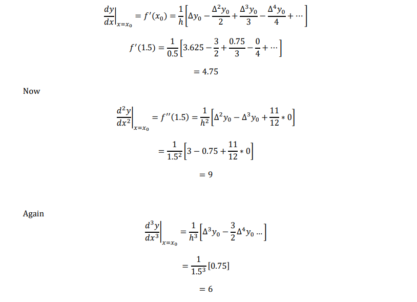
Example: find the first, second and third derivate of 𝑓(𝑥)𝑎𝑡 𝑥 = 1.5 if
| 𝑥 | 1.5 | 2.0 | 2.5 | 3.0 | 3.5 | 4.0 |
| 𝑓(𝑥) | 3.375 | 7.0 | 13.625 | 24 | 38.875 | 59.0 |
Solution
We have to find the derivate at the points 𝑥 = 1.5, which is at the beginning of the given data.
Therefore, we use the derivate of Newton’s Forward Interpolation formula.
Forward difference table is

ere 𝑥0 = 1.5, 𝑦0 = 3.375, ∆𝑦0 = 3.625, ∆ 2𝑦0 = 3, ∆ 3𝑦0 = 0.75, ∆ 4𝑦0 = 0, ℎ = 0.5
Now using equation for finding the derivate
Example:
The population of a certain town (as obtained from central data) is shown in the following table
| Year | 1951 | 1961 | 1971 | 1981 | 1991 |
| population (thousand) | 19.36 | 36.65 | 58.81 | 77.21 | 94.61 |
Find the rate of growth of the population in the year 1981
Solution
Here we have to find the derivate at 1981 which is near the end of the table, hence we use the
derivative of Newtons Backward difference formula. The table if difference is as follows:
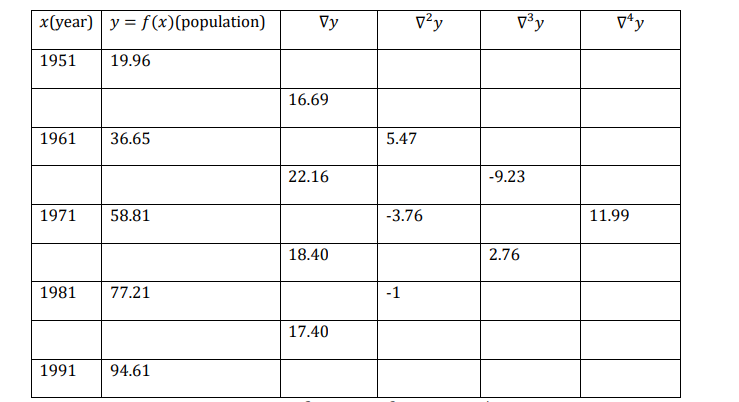
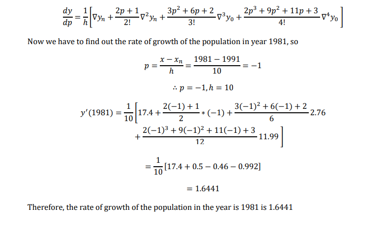
Here ℎ = 10, 𝑥𝑛 = 1991, ∇𝑦𝑛 = 17.4, ∇ 2𝑦𝑛 = −1, ∇ 3𝑦𝑛 = 2.76, ∇ 4𝑦𝑛= 11.99
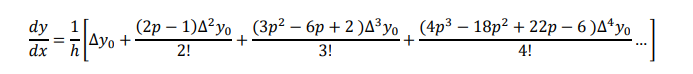
We know derivate for backward difference is
Maxima and minima of tabulated function
We know Newton’s forward interpolation formula as :
We know that maximum and minimum values of a function 𝑦 = 𝑓(𝑥) can be found by equating 𝑑𝑦/𝑑𝑥 to zero and solution for x

Now for keeping only up to third difference we have

Solving this for p, by substituting ∆𝑦0, ∆ 2𝑦0, ∆ 3𝑦0, we get 𝑥 as 𝑥0 + 𝑝ℎ at which y is a maximum or minimum
Example: given the following data, find the maximum value of y
| 𝑥 | -1 | 1 | 2 | 3 |
| 𝑦 | -21 | 15 | 12 | 3 |
Since the arguments (x -points) aren’t equally spaced we use Newton’s Divided Difference formula
𝑦(𝑥) = 𝑎0 + 𝑎1 (𝑥 − 𝑥0 ) + 𝑎2 (𝑥 − 𝑥0 )(𝑥 − 𝑥1 ) + 𝑎3 (𝑥 − 𝑥0 )(𝑥 − 𝑥1 )(𝑥 − 𝑥2 )…
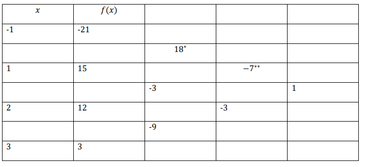
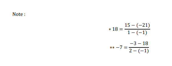
From above table 𝑎0 = −21, 𝑎1 = 18, 𝑎2 = −7, 𝑎3 = 1,
𝑓(𝑥) = −21 + 18(𝑥 + 1) + (𝑥 + 1)(𝑥 − 1)(−7) + (𝑥 + 1)(𝑥−1)(𝑥 − 2)(1) 𝑓(𝑥) = 𝑥 3 − 9𝑥 2 + 17𝑥 + 6
For maxima and minima 𝑑𝑦/𝑑𝑥 = 0
3𝑥 2 − 18𝑥 + 17 = 0
On solving we get
𝑥 = 4. .8257 𝑜𝑟 1.1743
Since x=4.8257 is out of range [-1 to 3] , we take x=1.1743
∴ 𝑦𝑚𝑎𝑥 = 𝑥 3 − 9𝑥 2 + 17𝑥 + 6
= 1.17433 − 9 ∗ 1.17342 + 17 ∗ 1.1743 + 6
= 15.171612
Differentiating continuous function
If the process of approximating the derivative 𝑓′(𝑥) of the function f(x), when the function itself is
available
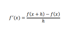
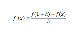
Forward Difference Quotient
Consider a small increment ∆𝑥 = ℎ in x, according to Taylor’s theorem, we have

Equation 3 is called first order forward difference quotient. This is also known as two-point formula.
The truncation error is in the order of h and can be decreased by decreasing h.
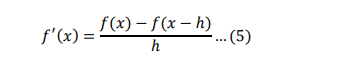
Similarly, we can show that the first order backward difference quotient is
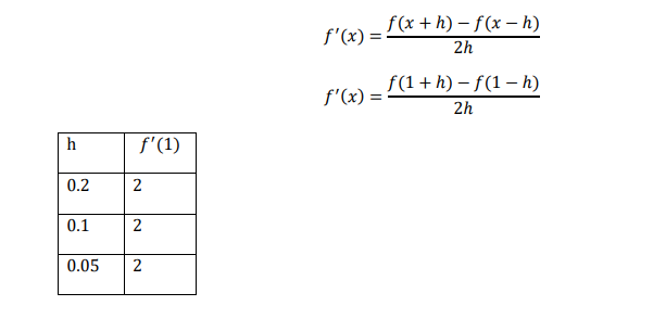
Central Difference Quotient
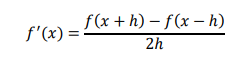
This equation is called second order difference quotient. Note that this is the average of the forward
difference quotient and backward difference equation. This is also called as three-point formula.
Example: estimate approximate derivative of 𝑓(𝑥) = 𝑥 2 𝑎𝑡 𝑥 = 1, for h=0.2,0.1,0.05 and 0.01, using first order forward difference formula
We know that
Derivative approximation is tabulated below as:
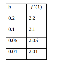
Note that the correct answer is 2. The derivative approximation approaches the exact value as h
decreases.
Now for central difference quotient
Numerical Integration

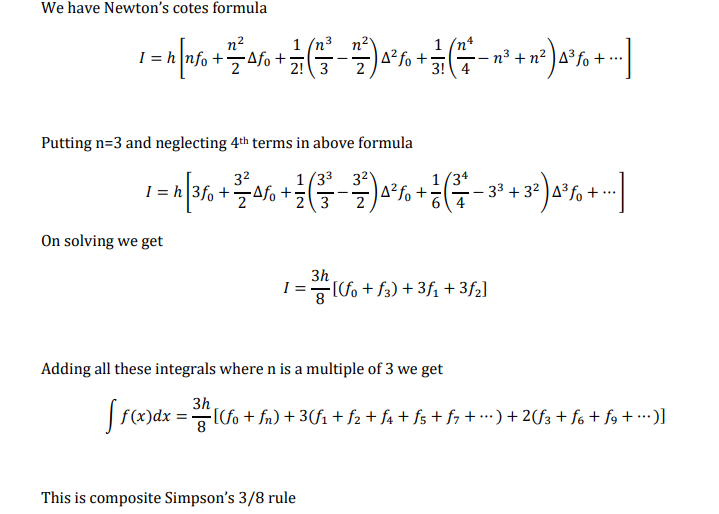
Newtons Cotes Formula
This is the most popular and widely used in numerical integration.
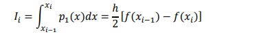
Numerical integration method uses an interpolating polynomial 𝑝𝑛(𝑥) in place of f(x)

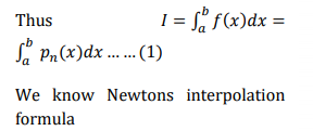

Above equation is known as Newton’s Cote’s quadrature formula, used for numerical integration
If the limits of integration a and b are in the set of interpolating points xi=0,1,2,3…..n, then the formula
is referred as closed form. If the points a and b lie beyond the set of interpolating points, then the
formula is termed as open form. Since the open form formula is not used for definite integration, we
consider here only the closed form methods. They include:
- Trapezoidal rule
- Simpson’s 1/3 rule
- Simpson’s 3/8 rule
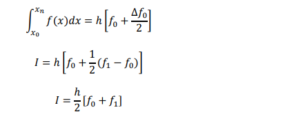
Trapezoidal rule (2 point formula)
Putting n=1 in equation 1 and neglecting second and higher order differences we get
Composite Trapezoidal Rule
If the range to be integrated is large, the trapezoidal rule can be improved by dividing the interval
(a,b) into a number of small intervals. The sum
of areas of all the sub-intervals is the integral of
the intervals (a,b) or (x0,xn). this is known as
composite trapezoidal rule.
As seen in the figure, there are n+1 equally spaced sampling point that create n segments of equal width h given by

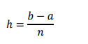
𝑥𝑖 = 𝑎 + 𝑖ℎ 𝑖 = 0,1,2, … n
From the equation of trapezoidal rule,
The total area of all the n segments is

Above equation is known as composite trapezoidal rule
Simpson’s 1 ⁄ 3 rule( 3 point formula)
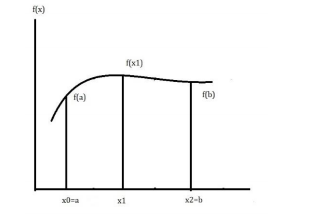
Another popular method is Simpson’s 1/3 rule. Here the function f(x) is approximated by second
order polynomial 𝑝2(𝑥) which passes through three sampling points as shown in figure. The three
points include the end point a & b and midpoint between 𝑥1 = (𝑎 + 𝑏)/2. The width of the segment
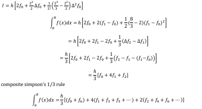
h is given by ℎ = (𝑏 − 𝑎)/𝑛 . Take n=2 and neglecting the third and higher order differences we get
(in newton’s cote formula)
Simpson’s 3/8 rule( 4 point rule)
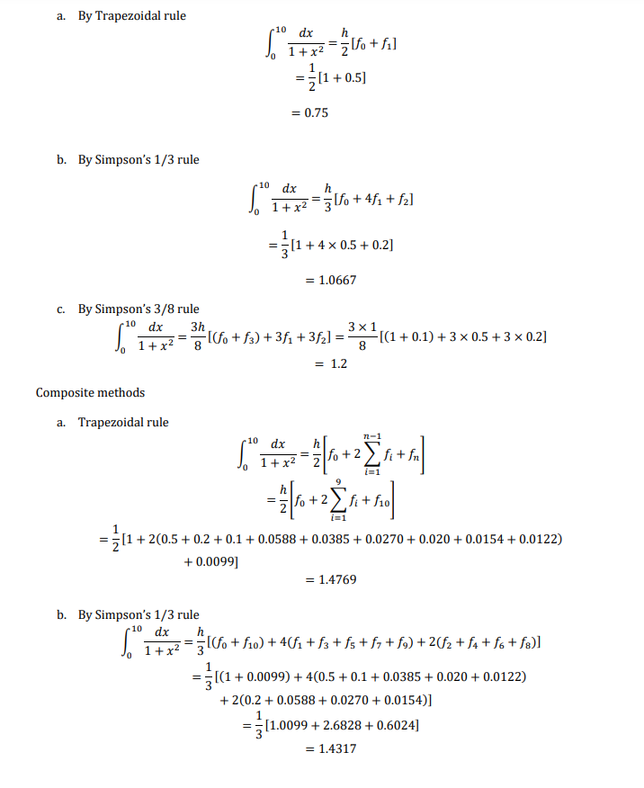
Example:
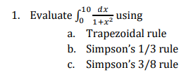
Solution
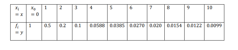
Taking h=1, divide the whole range of the integration [0,10] into ten equal parts. The value of the integrand for each point of sub division

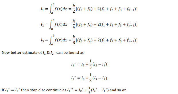
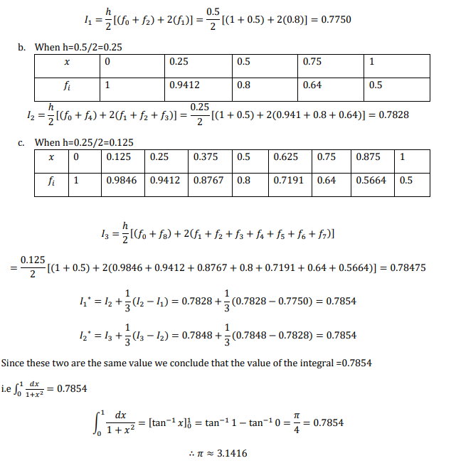
Romberg integration formula/ Richardson’s deferred approach to the limit or Romberg
method
Take an arbitrary value of h and calculate

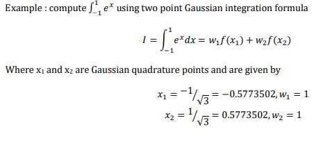
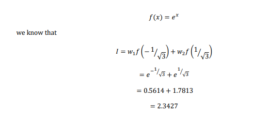
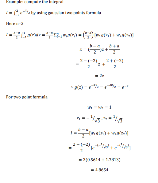
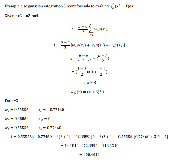
Gaussian integration
Gaussian integration is based on the concept that the accuracy of numerical integration can be improved by choosing sampling points wisely rather than on the basis of equal sampling. The problem is to compute the values of 𝑥1& 𝑥2 given the value of a and b and to choose approximate weights w1 & w2 . The method of implementing the strategy of finding approximate values of xi & wi and obtaining the integral of f(x) is called Gaussian integration or quadrature. Gaussian integration assumes an approximation of the form
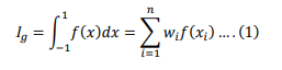
The above equation 1 contains 2n unknowns to be determined. For example for n=2, we need to find the values of w1,w2,x1,x2. We assume that the integral will be exact up to cubic polynomial. This implies the function x1,x2&x3 can be numerically integrated to obtain exact results.
Assume f(x)=1 (assume the integral is exact up to cubic polynomial)
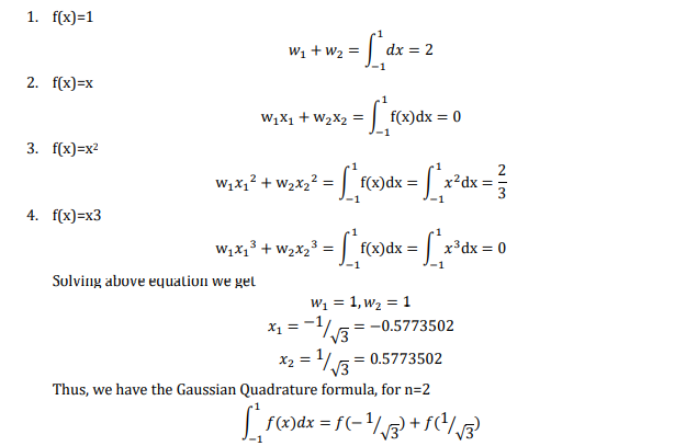
This formula will give correct value for the integral of f(x) in the range (-1,1) for any function
up to third order. The above equation is called gauss Legrendre formula
Changing limits of Integration
Note that the Gaussian formula imposed a restriction on the limits of integration to be from -1 to 1.
The restriction can be overcome by using the techniques of the “interval transformation” used in
calculus, let
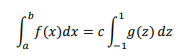
Assume the following transformation between x and new variable z. by following relation.
i.e x=Az+B
this must satisfy the following conditions at x=a, z=-1 & x=b, z=1
i.e B-A=a, A+B=b
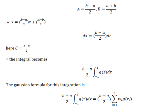
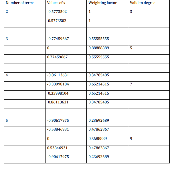
Where wi and zi are the weights and quadrature points for the integration domain (-1,1)
Values for gaussian quadrature
Reference 1 : Numerical Methods , Dr. V.N. Vedamurthy & Dr. N. Ch. S. N. Iyengar, Vikas Publishing House.
Good, also include En(x)=f^(n+1)[§]π{×-hx}/(n+1)!
And it’s differentiation.
That is error term in Newton forward difference