Solution of Linear Algebraic Equations: Matrices and their properties, Elimination and Gauss Jordan methods, Method of factorization, power, iterative

Matrices and properties

Importance of linear equations

First mathematical models of many of the real world problems are either linear or can be
approximated reasonably well using linear relationships. Analysis of linear relationship of variables
is generally easier than that of non-linear relationships.
A linear equation involving two variables x and y has the standard form 𝑎𝑥 + 𝑏𝑦 = 𝑐, where a, b&
c are real numbers and a and b both cannot be equal to zero.
The equation becomes non-linear if any of the variables has the exponent other than one, example

4𝑥 + 5𝑦 = 15 𝑙𝑖𝑛𝑒𝑎𝑟

4𝑥 − 𝑥𝑦 + 5𝑦 = 15𝑛𝑜𝑛 – 𝑙𝑖𝑛𝑒𝑎𝑟

 𝑥 ² + 5𝑦 ² = 15 𝑛𝑜𝑛 − 𝑙𝑖𝑛𝑒𝑎r

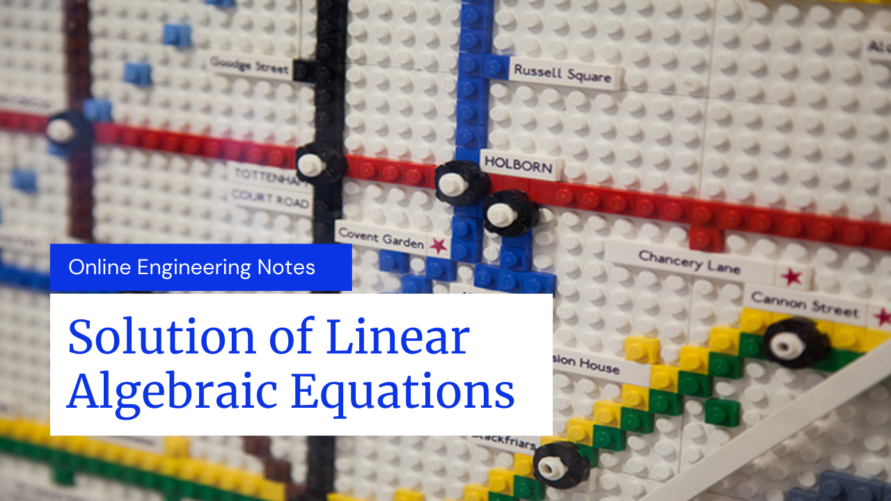
Linear equation occurs in more than two variables as 𝑎₁𝑥₁ + 𝑎₂𝑥₂ + 𝑎₃𝑥₃ + ⋯ 𝑎_𝑛𝑥_𝑛 = 𝑏. The set of equations is known as system of simultaneous equations, in matrix form it can be represented as

𝐴𝑥 = 𝐵

3𝑥₁ + 2𝑥₂ + 4𝑥₃ = 14

𝑥₁ − 2𝑥₂ = −7

 −𝑥₁ + 3𝑥₂ + 2𝑥₃ = 2

Existence of solution

In solving system of equations we find values of variables that satisfy all equations in the system
simultaneously. There may be 4 possibility in solving the equations.

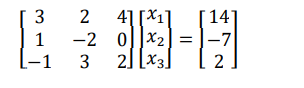
1. System with unique solution
   here the lines or equations intersect in one and only one point.

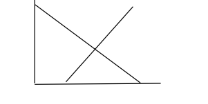
2. System with no solution
Here the lines or equation never intersect or parallel lines.

3. System with infinite solution

Here two equation or lines overlap, so that there is infinite
Solutions

4. ILL condition system

There may be situation where the system has a solution but it is very close to being
singular, i.e, any equation have solution but is very difficult to identify the exact point at
which the lines intersect. If there is any slight changes in the value in the equation then we
will see huge change in the solution, this type of equation is called ILL condition system,
we should be careful in solving these kind of solutions. Example

1.01𝑥 + 0.99𝑦 = 2
0.99𝑥 + 1.01𝑦 = 2

On solving these equations we get the solution at x=1 & y=1, however if we make small
changes in b i.e.

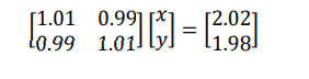
1.01𝑥 + 0.99𝑦 = 2.02
0.99𝑥 + 1.01𝑦 = 1.98

On solving these equation we get x=2 & y=0
So slight changes results in huge change in solution.

Methods of solutions

Elimination method

Elimination method is a method of solving simultaneous linear. This method involves elimination
of a term containing one of the unknowns in all but one equation, one such step reduces the order
of equations by one, repeated elimination leads finally to one equation with one unknown.
Example: solve the following equation using elimination method

4𝑥₁ − 2𝑥₂ + 𝑥₃ = 15 … … (1)

−3𝑥₁ − 𝑥₂+4𝑥₃ = 8 … … (2)

 𝑥₁ − 𝑥₂ + 3𝑥₃ = 13 … … (3)

Here multiply 𝑅₁ 𝑏𝑦 3 &𝑅₂ 𝑏𝑦 4 and add to eliminate 𝑥₁from 2. Multiply 𝑅₁ 𝑏𝑦 − 1&𝑅₃ 𝑏𝑦 4 and add to eliminate 𝑥₁from 3

4𝑥₁ − 2𝑥₂ + 𝑥₃ = 15

−10𝑥₂+19𝑥₃ = 77

−2𝑥₂ + 11𝑥₃ = 37

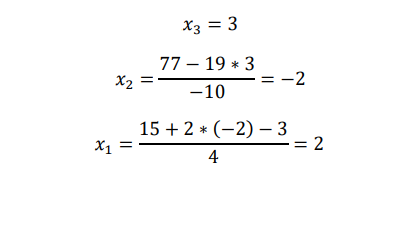
Now to eliminate 𝑥₂ from third equation multiply second row by 2 and third row by -10 and adding

4𝑥₁ − 2𝑥₂ + 𝑥₃ = 15

 −10𝑥₂+19𝑥₃ = 77

−72𝑥₃ = −216

Now we have a triangular system and solution is readily obtained from back-substitution

Gauss Elimination Method

The procedure in above example may not be satisfactory for large systems because the transformed coefficients can become very large as we convert to a triangular system. So we use another method called Gaussian Elimination method that avoid this by subtracting 𝑎𝑖1/ 𝑎11 times the first equation from 𝑖 ^𝑡ℎ equation to make the transformed numbers in the first column equal to zero and proceed on. However we must always guard against divide by zero, a useful strategy to avoid divide by zero is to re-arrange the equations so as to put the coefficient of large magnitude on the diagonal at each step, this is called pivoting. Complete pivoting method require both row and column interchange but this is much difficult and not frequently done. Changing only row called partial pivoting which places a coefficient of larger magnitude on the diagonal by row interchange only. This will be guaranteeing a non-zero divisors if there is a solution to set of equations and will have the added advantage of giving improved arithmetic precision. The diagonal elements that result are called pivot elements.

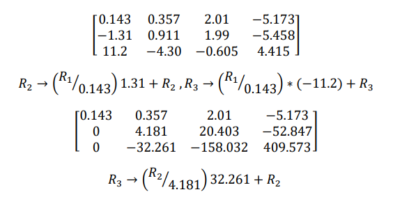
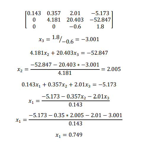
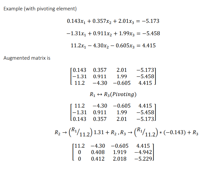
Example (without pivoting element)

0.143𝑥₁ + 0.357𝑥₂ + 2.01𝑥₃ = −5.173

−1.31𝑥₁ + 0.911𝑥₂ + 1.99𝑥₃ = −5.458

11.2𝑥₁ − 4.30𝑥₂ − 0.605𝑥₃ = 4.415

Augmented matrix is

Gauss Jordan Method

Gauss Jordan method is another popular method used for solving a system of linear equations. In
this method the elements above the diagonal are made zero at the same time that zero are
created below the diagonal, usually the diagonal elements are made ones at the same time the
reduction is performed, this transforms the coefficient matrix into identity matrix. When this has
been accomplished the column of right-hand side has been transformed into the solution vector.
Pivoting is normally employed to preserve arithmetic accuracy.

Example solution using Gauss-Jordan method

2𝑥₁ + 4𝑥₂ − 6𝑥₃ = −8

𝑥₁ + 3𝑥₂ + 𝑥₃ = 10

2𝑥₁ − 4𝑥₂ − 2𝑥₃ = −12

Example solution using Gauss-Jordan method (with pivoting)

2𝑥₁ + 4𝑥₂ − 6𝑥₃ = −8

𝑥₁ + 3𝑥₂ + 𝑥₃ = 10

2𝑥₁ − 4𝑥₂ − 2𝑥₃ = −12

Augmented matrix is

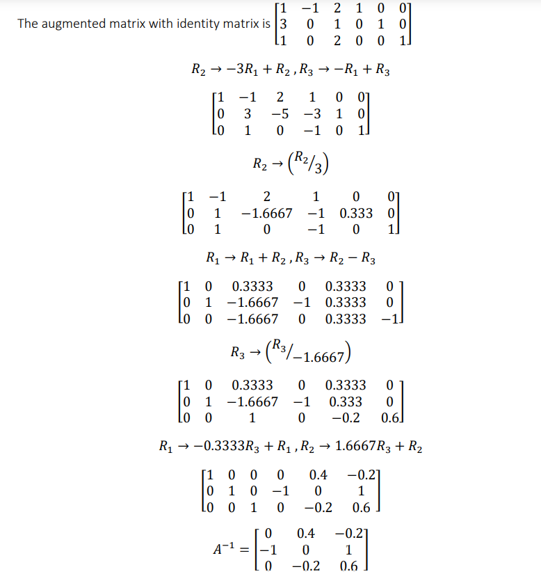
The inverse of a matrix

The division a matrix is not defined but the equivalent is obtained from the inverse of the matrix. If the product of two square matrices A*B equals identity matrix I, B is said to be inverse of A (also A is inverse of B). the usual notation of the matrix is 𝐴 ⁻¹ . we can say as 𝐴𝐵 = 𝐼, 𝐴 = 𝐵 ⁻¹ ,𝐵 = 𝐴 ⁻¹ .

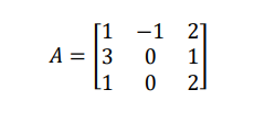
Example: given matrix A, find the inverse of A using Gauss Jordan method.

Method of factorization

Consider the following system of equations

𝑎₁₁𝑥₁ + 𝑎₁₂𝑥₂ + 𝑎₁₃𝑥₃ = 𝑏₁

 𝑎₂₁𝑥₁ + 𝑎₂₂𝑥₂ + 𝑎₂₃𝑥₃ = 𝑏₂

𝑎₃₁𝑥₁ + 𝑎₃₂𝑥₂ + 𝑎₃₃𝑥₃ = 𝑏₃

These equations can be written in matrix form as
𝐴𝑋 = B

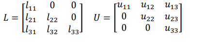
n this method we use the fact that the square matrix A can be factorized into the form LU, where
L is lower triangular matrix and U can be upper triangular matrix such that 𝐴 = 𝐿𝑈

𝐿𝑈𝑋 = 𝐵

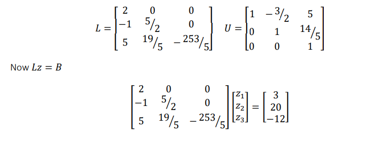
Let us assume 𝑈𝑋 = 𝑍 , then 𝐿𝑍 = 𝐵
Now we can solve the system A𝑋 = 𝐵 in two stages

1. Solve the equation, 𝐿𝑍 = 𝐵 for Z by forward substitution
2. Solve the equation, 𝑈𝑋 = 𝑍 for X using Z by backward substitution.

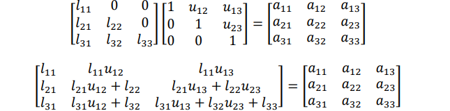
The elements of L and u can be determined by comparing the elements of the product of L and U
with those of A. The decomposition with L having unit diagonal values is called the Dolittle LU
decomposition while the other one with U having unit diagonal elements is called Crout LU
decomposition.

Dolittle LU decomposition

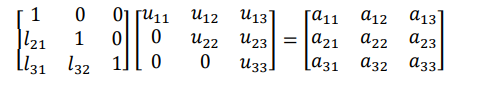
Equating the corresponding coefficients we get the values of l and u

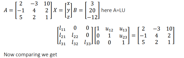
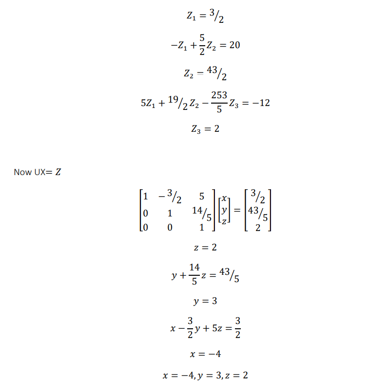
Example: Now find L & U either by using Dolittle algorithm

2𝑥 − 3𝑦 + 10𝑧 = 3
−𝑥 + 4𝑦 + 2𝑧 = 20
5𝑥 + 2𝑦 + 𝑧 = −12

The given system is 𝐴𝑥 = 𝐵, where

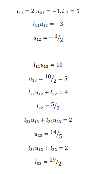
Now comparing both sides we get

𝑢₁₁ = 2

 𝑢₁₂ = −3

𝑢₁₃ = 10

𝑙₂₁𝑢₁₁ = −1

𝑙₂₁ = − 1/ 2

𝑙₂₁𝑢₁₂ + 𝑢₂₂ = 4

𝑢₂₂ = 5/ 2

𝑙₂₁𝑢₁₃ + 𝑢₂₃ = 2

𝑢₂₃ = 7

𝑙₃₁𝑢₁₁ = 5

𝑙₃₁ = 5/ 2

𝑙₃₁𝑢₁₂ + 𝑙₃₂𝑢₂₂ = 2

𝑙₃₂ = 19 /5

𝑙₃₁𝑢₁₃ + 𝑙₃₂𝑢₂₃ + 𝑢₃₃ = 1

𝑢₃₃ = − 253/ 5

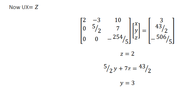
2𝑥 − 3𝑦 + 10𝑧 = 3
𝑥 = −4

Crout’s method

Equating the corresponding coefficients, we get the values of l and u

Example solve the following system by the method of crouts algorithms factorization
2𝑥 − 3𝑦 + 10𝑧 = 3
−𝑥 + 4𝑦 + 2𝑧 = 20
5𝑥 + 2𝑦 + 𝑧 = −12

The given system is 𝐴𝑥 = 𝐵, where

𝑙₃₁𝑢₁₃ + 𝑙₃₂𝑢₂₃ + 𝑙₃₃ = 1

𝑙₃₃ = − 253/ 5

So we have

Choleskys method

In case of A is symmetric, the LU decomposition can be modified so that upper factor in matrix is
the transpose of the lower one (vice versa)
i.e. 𝐴 = 𝐿𝐿 ^𝑇 = 𝑈 ^𝑇 𝑈

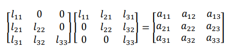
Just as other method, perform as before

Symmetric matrix

A square matrix 𝑨 = [𝒂_𝒊𝒋] is called symmetric if 𝒂_𝒊𝒋= 𝒂_𝒋𝒊 for all i and j

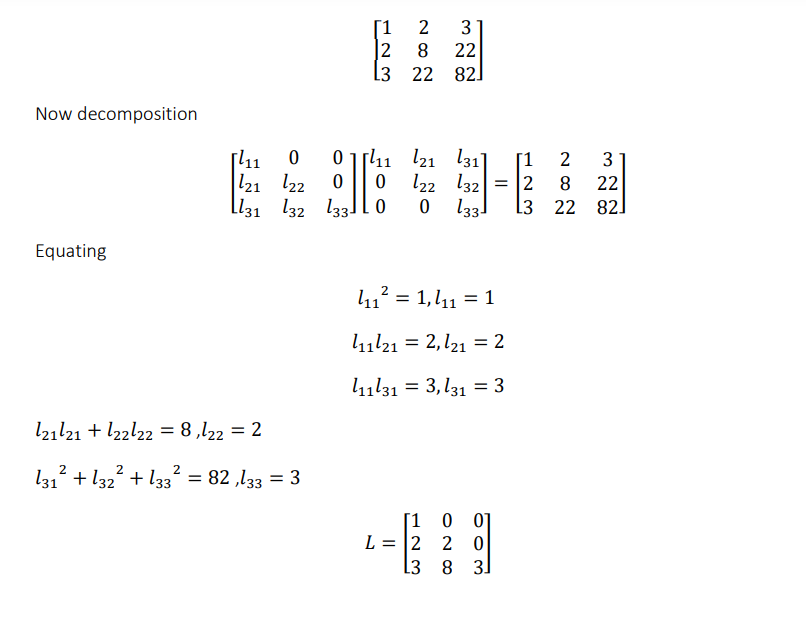
Example: factorize the matrix, using Cholesky algorithm

Iterative methods

Gauss elimination and its derivatives are called direct method, an entirely different way to solve
many systems is through iteration. In this we start with an initial estimate of the solution vector
and proceed to refine this estimate.
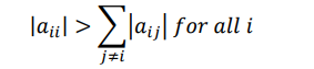
When the system of equation can be ordered so that each diagonal entry of the coefficient matrix
is larger in magnitude that the sum of the magnitude of the other coefficients in that row, then
such system is called diagonally dominant and the iteration will converge for any stating values.
Formally we say that an nxn matrix A is diagonally dominant if and only if for each i=1, 2, 3….n

The iterative method depends on the arrangement of the equations in this manner
Let us consider a system of n equations in n unknowns

𝑎₁₁𝑥₁ + 𝑎₁₂𝑥₂ + ⋯ + 𝑎_1𝑛𝑥_𝑛 = 𝑏₁

𝑎₂₁𝑥₁ + 𝑎₂₂𝑥₂ + ⋯ + 𝑎_2𝑛𝑥_𝑛 = 𝑏₂

𝑎_𝑛1𝑥₁ + 𝑎_𝑛2𝑥₂ + ⋯ + 𝑎_𝑛𝑛𝑥_𝑛= 𝑏_𝑛

We write the original system as

Now we can computer 𝑥₁, 𝑥₂ … 𝑥_𝑛by using initial guess for these values. The new values area gain used to compute the next set of x values. The process can continue till we obtain a desired level of accuracy in x values.

Example
Solve the equation using Gauss Jacobi iteration method

6𝑥₁ − 2𝑥₂ + 𝑥₃ = 11

𝑥₁ + 2𝑥₂ − 5𝑥₃ = −1

−2𝑥₁ + 7𝑥₂ + _2𝑥3 = 5

Now first we recorder the equation so that coefficient matrix is diagonally dominant

6𝑥₁ − 2𝑥₂ + 𝑥₃ = 11

−2𝑥₁ + 7𝑥₂ + 2𝑥₃ = 5

 𝑥₁ + 2𝑥₂ − 5𝑥₃ = −1

Now

We can simplify as

We begin with some initial approximation to the value of the variables,

 let’s take as 𝑥₁ = 0, 𝑥₂ = 0, 𝑥₃ = 0,

Then new approximation using above formula will be as follows

1 Iteration

𝑥1=1.833333

𝑥2=0.714286

𝑥3=0.200000

2 Iteration

𝑥1=2.038095

𝑥2 =1.180952

𝑥3=0.852381

3 Iteration

𝑥1=2.084921

𝑥2=1.053061

𝑥3=1.080000

4 Iteration

𝑥1=2.004354

𝑥2=1.001406

𝑥3=1.038209

5 Iteration

𝑥1=1.994100

𝑥2=0.990327

𝑥3=1.001433

6 Iteration

𝑥1=1.996537

𝑥2=0.997905

𝑥3=0.994951

7 Iteration

𝑥1=2.000143

𝑥2=1.000453

𝑥3=0.998469

8 Iteration

𝑥1=2.000406

𝑥2=1.000478

𝑥3=1.000210

9 Iteration

𝑥1=2.000124

𝑥2=1.000056

𝑥3=1.000273

10 Iteration

𝑥1=1.999973

𝑥2=0.999958

𝑥3=1.000047

11 Iteration

𝑥1=1.999978

𝑥2=0.999979

𝑥3=0.999978

12 Iteration

𝑥1=1.999997

𝑥2=1.000000

𝑥3=0.999987

12 Iteration the final result is :

𝑥1=1.999997 𝑥2=1.000000 𝑥3=0.999987

Gauss Seidel Iteration method

This is a modification of Gauss Jacobi method, as before

Let us consider a system of n equations in n unknowns

 𝑎₁₁𝑥₁ + 𝑎₁₂𝑥₂ + ⋯ + 𝑎_1𝑛𝑥_𝑛 = 𝑏₁

𝑎₂₁𝑥₁ + 𝑎₂₂𝑥₂ + ⋯ + 𝑎_2𝑛𝑥_𝑛 = 𝑏₂

𝑎_𝑛1𝑥₁ + 𝑎_𝑛2𝑥₂ + ⋯ + 𝑎_𝑛𝑛𝑥_𝑛 = 𝑏₃

We write the original system as

Now we can computer 𝑥₁, 𝑥₂ … 𝑥_𝑛 by using initial guess for these values. Here we use the updated values of 𝑥₁, 𝑥₂ … 𝑥_𝑛 in calculating new values of x in each iteration till we obtain a desired level of accuracy in x values. This method is more rapid in convergence than gauss Jacobi method. The rate of convergence of gauss seidel method is roughly twice that of gauss Jacobi.

Example
Solve the equation using Gauss Seidel iteration method

8𝑥₁ − 3𝑥₂ + 2𝑥₃ = 20

 6𝑥₁ + 3𝑥₂ + 12𝑥₃ = 35

4𝑥₁ + 11𝑥₂ − 𝑥₃ = 33

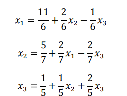
Now first we recorder the equation so that coefficient matrix is diagonally dominant

8𝑥₁ − 3𝑥₂ + 2𝑥₃ = 20

4𝑥₁ + 11𝑥₂ − 𝑥₃ = 33

 6𝑥₁ + 3𝑥₂ + 12𝑥₃ = 35

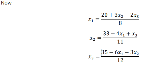
We begin with some initial approximation to the value of the variables,

let’s take as 𝑥₂ = 0, 𝑥₃ = 0,

Then new approximation using above formula will be as follows

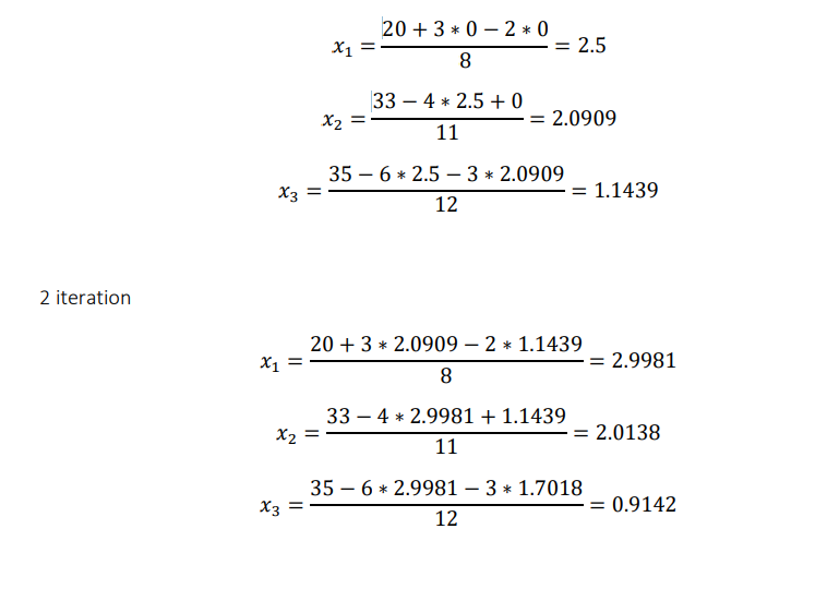
Since the 6^th and 7^th approximate are almost same up to 4 decimal places, we can the result is

 𝑥₁ = 3.0168, 𝑥₂ = 1.9859, 𝑥₃ = 0.9118

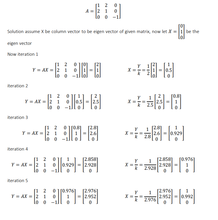
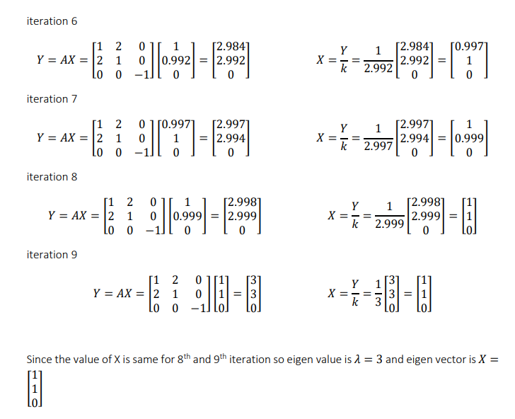
Power method
Power method is a single value method used for determining the dominant eigen value of a matrix.
It as an iterative method implemented using an initial starting vector x. the starting vector can be
arbitrary if no suitable approximation is available. Power method is implemented as follows
𝑌 = 𝐴𝑋 − − − − − (𝑎)

𝑋 = 𝑌/𝑘 − − − − − (𝑏)
The new value of X is obtained in b is the used in equation a to compute new value of Y and the
process is repeated until the desired level of accuracy is obtained. The parameter k is called scaling
factor is the element of Y with largest magnitude.

Example: find the largest Eigen value 𝜆 and the corresponding vector v, of the matrix using power
method

Reference 1 : Numerical Methods , Dr. V.N. Vedamurthy & Dr. N. Ch. S. N. Iyengar, Vikas Publishing House.