Turbulent flow : Prandtl’mixing length theory, Darcy-Weisbach equation, Nikuradse’ experiment, Colebrook-White and use of Moody’s diagram

Turbulent Flow:

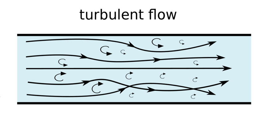
Turbulent flow is defined as that type of flow in which the fluid particles move in zigzag way. The fluid particle crosses the paths of each other. The Reynolds number (Re) is greater than 4000 then the flow is said to be turbulent.

For example:

a. Flow in river at the time of flood.

b. Flow through pipe of different cross sections.

Difference between Laminar and Turbulent flow:

Laminar Flow	Turbulent Flow
1. All the fluid layer move parallel to each other and do not cross one another.	1. Fluid layers cross each other and donot move parallel.
2. Generally it occurs in small diameter pipe and flow at low velocity.	2. Almost all high velocity and very large diameter pipe flow are turbulent flow.
3. The flow velocity profile is parabolic and the maximum velocity is at centre of the pipe line.	3. The velocity profile is almost flat across the centre section of the pipe and drops rapidly extremely close to the wall.
4. The average flow velocity is approximately one half of the maximum velocity.	4. The average flow velocity is approximately equal to the velocity at the centre of the pipe.
5. The value of Reynolds number is less than 2000.	5. The value of Reynolds number is above 4000.

Shear stress in Turbulent flow:

The shear stress in viscous flow is given by Newton law of viscosity as

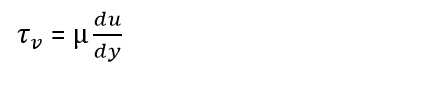
Where,

𝝉_v = Shear stress due to velocity.

Similarly, Turbulent shear stress ( by J. Boussineq) is expressed as

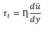
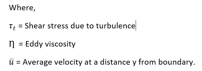
The ratio of η (eddy viscosity) and ρ (mass density) is known as kinematic eddy viscosity and is denoted by ε.

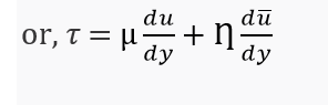
If the shear stress due to viscous flow is also considered, then the total shear stress becomes

𝜏 = 𝜏_v + 𝜏_t

The value of  η = 0 for laminar flow. For other case the value of η may be serveral thousand times the value of μ.

Prandtl’s mixing length theory:

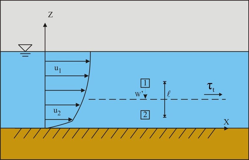
According to Prandtl, the mixing length L, is that distance between two layers in the transverse direction such that the lumps of the fluid particles from one layer could reach the other layer and the particles are mixed in the other layer in such a way that the lumps of the fluid particles from one layer could reach the other layer and the particles are mixed in the other layer in such a way that the momentum of the particles in the direction of x is same. It is assumed that the velocity fluctuation in the x-direction  u^| is related to the mixing length L as

u^| = L * du/ dy

And,

v^| is the fluctuation components of velocity in y-direction is of the same order of magnitude as u^| and hence,

v^| = L du/dy

Now,

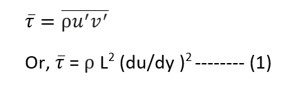
u^| * v^| = u^| * v^|

or, u^| * v^|  = (L * du/ dy) *( L * du/ dy)

or, u^| * v^|   = L² (du/dy )²

Substituting the value of u^| * v^|  in equation of turbulent shear stress, we get the expression for shear stress in turbulent flow due to Prandtl’s  as

Thus,

The total shear stress at any point in turbulent flow is the sum of shear stress due to viscous shear and can be written as

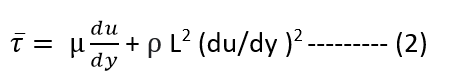
Equation (2) is the general expression for shear stress distribution for turbulent flow in circular pipe.

Velocity Distribution

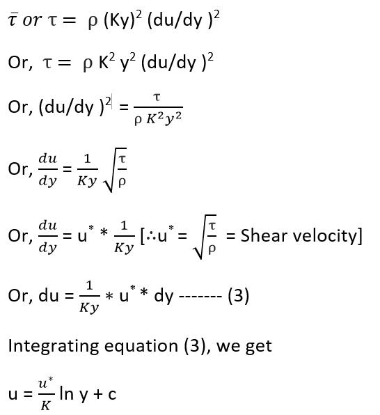
Prandtl assumed that the mixing length L is a linear function of the distance y from the pipe wall i.e.

L=Ky

Where, K is a constant known as Karman constant = 0.4

Substituting the value of L in equation (1) , we get

Using Boundary conditions

Y=R

u= U_max

[∴ K = 0.4 = Karman constant]

Or, u = U_max +2.5 u^* ln (y/R) ————–(4)

Above expression is called Prandtl universal velocity distribution for turbulent flow through pipe.

Dividing equation (4) by u^*, we get

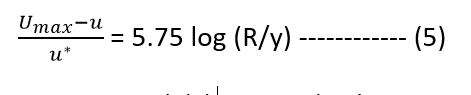
In equation (5) ( U_max – u ) is known as velocity defect.

Darcy-Weisbach equation

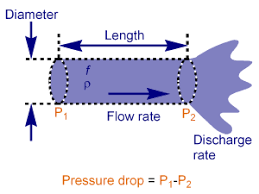
Consider a uniform horizontal pipe having steady flow as shown above figure. Also, consider 1-1 and 2-2 are two sections of pipe.

Let,

P₁ = Pressure intensity at sections 1-1

P₂ = Pressure intensity at sections 2-2

v₁ = Velocity of flow at section 1-1

v₂ = Velocity of flow at section 2-2

L =  Length of the pipe between section 1-1 and 2-2

d = Diameter of pipe

f^| = Frictional resistance per unit wetted area per unit velocity

hf =  Loss of head due to friction

Applying Bernoulli’s equation between sections 1-1 and 2-2

Total head at 1-1 = Total head at 2-2 + loss of head due to friction between 1-1 and 2-2

But,

z₁ = z₂ as pipe is horizontal

v₁ = v₂ as diameter of pipe is same at 1-1 and 2-2

But, hf is the head loss due to friction and hence intensity of pressure will be reduced in the direction of flow by frictional resistance.

Now,

Frictional resistance = Frictional resistance per unit wetted area per unit velocity * wetted area * velocity²

Or, F₁ = f^| * π dL * v²

[∴ Wetted area = π dL, Velocity = v = v₁=v₂]

Or, F₁ = f^| *P*L*v² ————–(2)

[∴π d = Perimeter = P ]

The forces acting on the fluid between sections 1-1 and 2-2 are:

• Pressure force at section 1-1 = P₁ * A

where, A= Area of pipe

• Pressure force at sections 2-2 = P₂ *A
• Frictional force F₁ as shown in figure.

Resolving all forces in the horizontal direction, we have

P₁A- P₂A – F = 0 ————-(3)

Or, (P₁ – P₂ )A = F₁ = f^| * P *L*v²

[∴ From eqaution (2), F₁ = f^| PLv² ]

Or, P₁ – P₂ = (f^| PLv²)/A

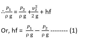
But, from equation (1), P₁ – P₂ = ρgh_f

Equating the value of ( P₁ – P₂), we get

ρgh_f = (f^| PLv²)/A

or, h_f = (f^| /ρg) *(P/A)*L* v² ————-(4)

In equation (4)

P/A = Wetted perimeter/ Area

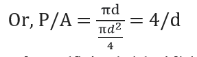
∴ h_f = (f^| /ρg) *(4/d)*L* v²

Or, h_f = (f^| /ρg) *(4Lv² /d)—————-(5)

Putting f^| /ρ = f/2

Where, f is known as coefficient of friction.

Equation becomes as

h_f = (4f/2g) * (Lv²/d)

or, h_f = (4f Lv²)/ (d*2g) ————–(6)

Equation (6) is known as Darcy Weisbach eqaution.

Also, equation(6) is written as

h_f = (fLv²) / d* 2g

Then, f is known as friction factor.

Nikuradse’s experiment:

He coated several different size of pipe with sand grains that had been sorted by sieving so as to obtain different sizes of grains of reasonably conform diameter. The diameter of grain sand grains may be represented by e, which is known as absolute roughness, e/d is relative roughness, where d is diameter of pipe.

The test results are plotted graphically as shown in figure:

The grain shows following character:

• Laminar and turbulent flow regime is indicated by change in relation between f and Re.
• Laminar regime is characterized by a single curve f= 64/Re for all roughness.
• In turbulent flow, curve of f versue Re exists for every relative roughness, e/d.
• At high Reynolds number friction factor becomes constant.

Friction coefficient for commercial pipe:

According to Blasius, F= 0.3164/Re1/4

According to Pradtl, 1/F = 2 log₁₀ Re F^1/2 – 0.8 for smooth pipes

According to Karman, 1/F^1/2 =  1.14 + 2 log₁₀ D/e for turbulent flow

Colebook-white equation

1/F^1/2 = 0.86 ln Re F^1/2 – 0.8 , for smooth pipe flow

1/F^1/2 = -0.86 ln(e/3.70 + 2.5/ReF^1/2), for transion zone

1/F^1/2 = -0.86 ln(e/3.7D), for complete turbulent zone.

Moody Chart:

Moody chart may be divided into four zones:

• The laminar zone where friction factor is function of Reynolds number.
• Critical zone where values are uncertain.
• Transition zone, f is friction of Re and e/d ratio.
• Turbulent zone f is independent of Re and depends on only e/d.

Hydraulic Gradient and Total Energy Line:

1. Hydraullic Gradient Line:

It is defined as the line which gives the sum of pressure headd P/W and datum head(Z) of flowing fluid in a pipe with respect to some reference line or it is the line which is obtained by joining the top of all vertical ordinates showing the pressure head P/W of a flowing fluid in a pipe from the centre of the pipe.

2. Total Energy Line:

It is defined as the line which gives the sum of pressure head, datum head and kinetic head of a flowing fluid in a pipe with respect to some reference line. It is also defined as the line which is obtained by joining the tops of all vertical ordinates showing the sum of pressure head and kinetic head from the centre of the pipe.

Minor Head ( energy) Losses:

The minor loss of energy (or head) includes the following cases:

1. Loss of head due to sudden enlargement
2. Loss of head due to sudden contraction
3. Loss of head at the entrance of a pipe
4. Loss of head at the exit of a pipe
5. Loss of head due to an obraction in a pipe
6. Loss of head due to bend in the pipe
7. Loss of head in various pipe fittings