Solution of Ordinary Differential and Higher Order Equations: Overview of initial and boundary value problems & Taylor series, Euler, Huen’s and Runge-Kutta methods

Differential equations

Many of the laws in physics, chemistry, engineering, economics are based on empirical
observations that describe changes in the state of the system. Mathematical models that
describe the state of such system are often expressed in terms of not only certain system
parameters but also their derivatives, such mathematical model which uses differential
calculus to express relationship between variables are known as differential equations.
Examples:

Here
• The quantity y that is being differentiated is called dependent variable.
• The quantity with respect to which the dependent variable is differentiated is called
independent variable.
• If there is only one independent variable then the equation is called an ordinary
differential equation.
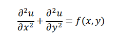
• If the equation contains more than one independent variable then it is called partial
differential equation

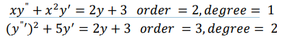
Order of equation
The highest derivative that appears in the equation is called order. If there is only first
derivative then it called first order differential equation.

Degree of equation
The degree of differential equation is the power of the highest order derivative

Initial value problem

In order to obtain the values of the integration constant, we need additional information for example consider the solution 𝑦 = 𝑎𝑒 ^𝑥 to the equation 𝑦 ′ = 𝑦. if we are giving a value of y for some x, the constant a can be determined, suppose y=1 when x=0, then 𝑦(0) = 𝑎𝑒 ⁰ = 1,

∴ 𝑎 = 1 and particular solution is 𝑦 = 𝑒 ^𝑥

It is also possible to specify the condition at different values of the independent variables such problems are called boundary value problem.

Example 𝑦 ” = 𝑓(𝑥, 𝑦, 𝑦 ′ ) 𝑦(𝑎) = 𝐴, 𝑦(𝑏) = 𝐵 𝑤ℎ𝑒𝑟𝑒 𝑎 & 𝑏 𝑎𝑟𝑒 𝑡𝑤𝑜 𝑑𝑖𝑓𝑓𝑒𝑟𝑒𝑛𝑡 𝑝𝑜𝑖𝑛𝑡𝑠.

Solution of ordinary differential equations

1. Taylor’s series method
2. Euler’s method
3. Heun’s method
4. Runge’s method
5. Runge’s Kutta 4th order method
6. Shooting method
7. Picard’s method
8. R.K method for simultaneous equations
9. Solution of higher order differential equation

Taylor’s series

Taylor series is often used in determining the order of errors for methods and the series itself is the basic for some numerical procedures.

 Let 𝑦 ′ = 𝑓(𝑥, 𝑦), 𝑦(𝑥₀ ) = 𝑦₀ (1)

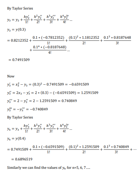
Be the differential equation to which the numerical solution is required. Expanding 𝑦(𝑥) about 𝑥 = 𝑥₀ by Taylor Series we get

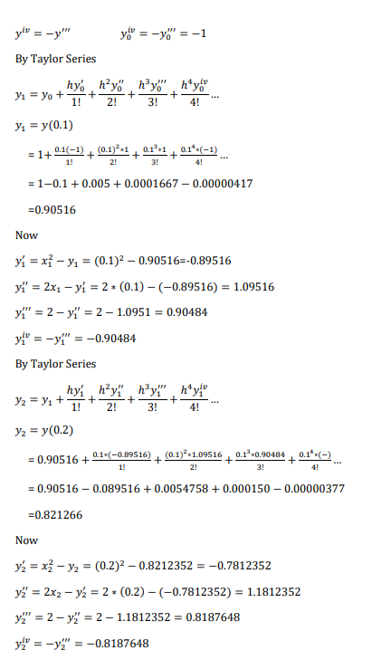
Here 𝑦₀ ′ , 𝑦₀ ′′ , 𝑦₀ ′′′ … can be found using equation (1) and its successive differentiation at 𝑥 = 𝑥₀. The series in (4) can be truncated at any stage if ‘h’ is small. Now having obtained 𝑦1we can calculate 𝑦₁ ′ , 𝑦₁ ′′ , 𝑦₁ ′′′ from equation (1) at 𝑥 = 𝑥₀ + h

 Now expanding 𝑦(𝑥) by Taylor series about 𝑥 = 𝑥₁, we get

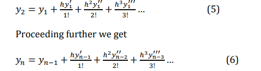
By taking sufficient number of terms in above series the value of 𝑦_𝑛can be obtained without much error

 If a Taylor series is truncated while there are still non-zero derivatives of higher order the truncated power series will not be exact. The error term for a truncated Taylor Series can be written in several ways but the most useful form when the series is truncated after 𝑛 ^𝑡ℎ term is

Where 𝜉 is a value between x and (x+a). the value of 𝜉 is ordinarily not known so there is
some uncertainty in the exact value of error still this term can give bounds for the errors.

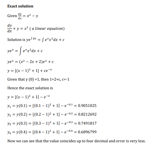
Example:

Euler’s method

Euler’s method is the simplest one step method. It has limited application because of its low
accuracy. From Taylor’s theorem we have

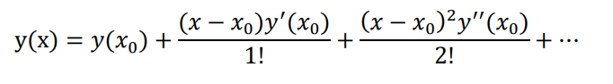
Taking only first two terms only 𝑦(𝑥) = 𝑦(𝑥₀ ) + 𝑦 ′ (𝑥₀ )(𝑥 − 𝑥₀ )

Now we get

 𝑦(𝑥₁ ) = 𝑦₁ = 𝑦(𝑥₀ ) + (𝑥₁ − 𝑥₀ )𝑓(𝑥₀, _𝑦0 )

where 𝑥 = 𝑥₁, 𝑓(𝑥₀, 𝑦₀ ) = 𝑦 ′ (𝑥₀ )

Now let ℎ = 𝑥₁ − 𝑥₀ 𝑦₁ = 𝑦₀ + ℎ𝑓(𝑥₀, 𝑦₀)

Similarly 𝑦₂ = 𝑦₁ + ℎ𝑓(𝑥₁, 𝑦₁)

In general 𝑦_𝑖+1 = 𝑦_𝑖 + ℎ𝑓(𝑥_𝑖 , 𝑦_𝑖)

This formula is known as Euler’s method and can be used recursively to evaluate y₁, y₂ … starting from the initial condition 𝑦₀ = 𝑦(𝑥₀)

• A new value of y is estimated using the previous value of y as initial condition.
• The term hf(x_i,y_i) represents the incremental value of y and f(x_i,y_i) is the slope of y(x) at (x_i,y_i), the new value is obtained by extrapolating linearly over the step size h using the slope at its previous value. i.e. new value =old value + slope x step size

Example : Given the equation 𝑦 ′ (𝑥) = 3𝑥 ² + 1, with y(1)=2, estimate y(2), using euler’s method using h=0.5 & h=0.25,

Solution 𝑦 ′ (𝑥) = 𝑓(𝑥, 𝑦) = 3𝑥 ² + 1

𝑦(1) = 2, 𝑦(𝑥₀ ) = 𝑦₀, 𝑥₀ = 1, 𝑦₀ = 2

We know that

𝑦_𝑖+1 = 𝑦_𝑖 + ℎ𝑓(𝑥_𝑖 , 𝑦_𝑖)

a. h=0.5

 𝑦₁ = 𝑦(₁ + 0.5) = 𝑦(1.5) = 𝑦₀ + ℎ𝑓(𝑥₀, 𝑦₀ ) = 𝑦(1) + 0.5 × (3 × 1 ² + 1) = 2 + 0.5 × 4 = 4

𝑦₁ = 𝑦(2.0) + 𝑦(1.5 + 0.5) = 𝑦₁ + ℎ𝑓(𝑥₁, 𝑦₁ ) = 𝑦(1.5) + 0.5 × 𝑓(𝑥_1.5, 𝑦_1.5 )

= 4 + 0.5 × (3 × 1.5 ² + 1)

= 7.8750

∴ 𝑦(2) = 7.8750

b. h=0.25

𝑦(1) = 2

𝑦₁ = 𝑦(1 + 0.25) = 𝑦(1.25) = 𝑦₀ + ℎ𝑓(𝑥₀, 𝑦₀ ) = 2 + 0.25 × 𝑓(1,2) = 2 + 0.25(3 × 1 ² + 1) = 3

 𝑦₂ = 𝑦(1.25 + 0.25) = 𝑦(1.5) = 𝑦₁ + ℎ𝑓(𝑥₁, 𝑦₁ ) = 3 + 0.25 × 𝑓(1.25,3) = 3 + 0.25(3 × 1.252 + 1) = 4.4218 𝑦₃ = 𝑦(1.5 + 0.25) = 𝑦(1.75) = 𝑦₂ + ℎ𝑓(𝑥₂, 𝑦₂ ) = 4.4218 + 0.25 × 𝑓(1.5,4.4218) = 4.4218 + 0.25(3 × 1.5 ² + 1) = 6.3593

 𝑦₄ = 𝑦(1.75 + 0.25) = 𝑦(2.0) = 𝑦₃ + ℎ𝑓(𝑥₃, 𝑦₃ ) = 6.3593 + 0.25 × 𝑓(1.75,6.3593) = 6.3593 + 0.25(3 × 1.752 + 1) = 8.9061

∴ 𝑦(2.0) = 8.9061

Heun’s method

Euler’s method is the simplest of all one step methods. It is easy to implement on computers.
One of the major weakness is large truncation error in Euler’s method. This is due to the fact
that Euler’s method uses only the first two terms of Taylor’s series. Now heun’s method also
called improved Euler’s method.

In Euler’s method the slope at the beginning of the interval is used to extrapolate yi to yi+1 over the entire interval, thus

𝑦_𝑖+1 = 𝑦_𝑖 + 𝑚₁ℎ. . . . . . . . 𝑎

where m₁ is the slope at(x_i,y_i).

Alternative is to use the line which is parallel to the tangent at the point [𝑥_𝑖+1, 𝑦(𝑥_𝑖+1 )] to extrapolate from 𝑦𝑖 𝑡𝑜 𝑦_𝑖+1

𝑦_𝑖+1 = 𝑦_𝑖+ 𝑚₂ℎ. . . . . . . . 𝑏

Where is m₂ is the slope at [𝑥_𝑖+1, 𝑦(𝑥_𝑖+1 )]. Note that the estimate appears to be overestimated.

Now a third approach is to use a line whose slope is the average of the slopes at the end
points of the interval, i.e

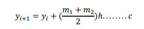
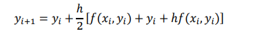
This gives the better approximation to 𝑦_𝑖+1, this approach is known as Heun’s method. The formula for implementing Heun’s method can be constructed easily as 𝑦 ′ (𝑥) = 𝑓(𝑥, 𝑦)

Note that the term y_i+1 appears on both sides. The value y_i+1 cannot be calculated until the value of y_i+1 inside the function f(x_i+1,y_i+1) is available. This value can be predicted using Eulers formula as

𝑦_𝑖+1 = 𝑦_𝑖 + ℎ𝑓(𝑥_𝑖 , 𝑦_𝑖)

Then the Heun’s formula can be written as:

Putting the value of euler’s formula in above equation we get

Example :

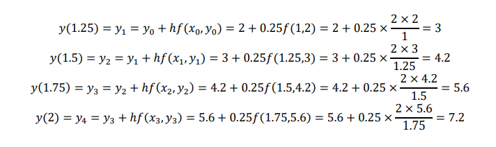
Given the equation 𝑦 ′ (𝑥) = 2𝑦/ 𝑥 with y(1)=2, estimate y(2) using 1) Euler’s method 2) Heun’s method and compare the result. Take h=0.25

Solution

.

I. Euler’s method
h=0.25, y(1)=2

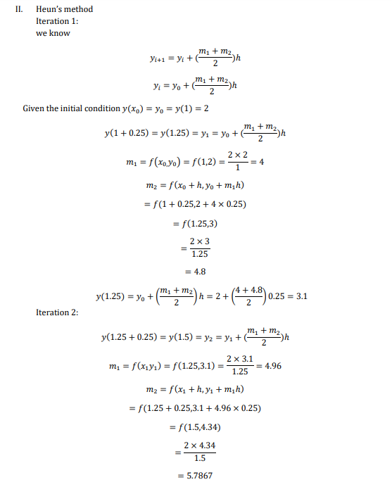
The above equation can be done using the following formula, note this is same
problem but done using later formula, you can use any method which ever you feel
easy to use.

Runge kutta method

 Runge Kutta Method refers to a family of one step methods used for numerical solution of initial value problems. They are all based on the general form of the extrapolation equation

𝑦_𝑖+1 = 𝑦_𝑖 + 𝑠𝑙𝑜𝑝𝑒 × 𝑖𝑛𝑡𝑒𝑟𝑣𝑎𝑙 𝑠𝑖𝑧𝑒 = 𝑦_𝑖 + 𝑚ℎ

Where m represents the slope that is weighted averages of the slope at various points in the interval h. Runge Kutta(RK) methods are known by their order. For instance an RK method is called r-order Runge Kutta method when slope at r points are used to construct the weighted average slope m.

Euler’s method is the first order RK method because it uses only one slope at (x_i,y_i) to estimate 𝑦_𝑖+1. Huen’s method is a second order RK method because it employs slope at two ends points of the interval. It demonstrated that higher order would be better the accuracy of estimates.

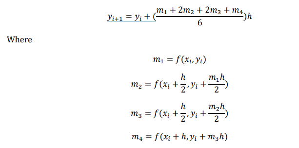
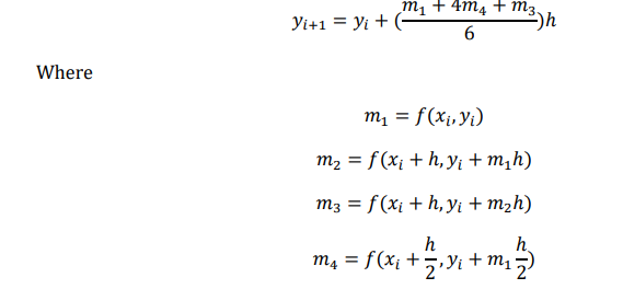
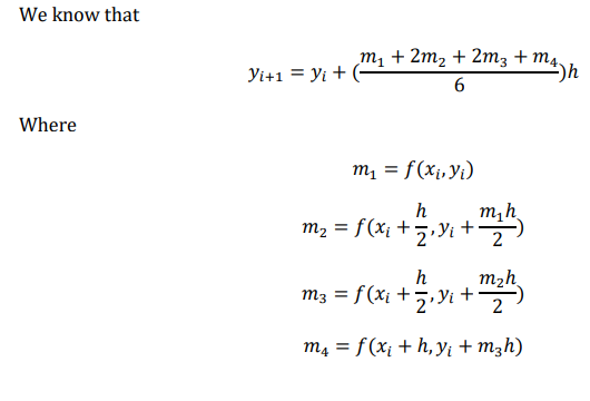
Fourth order Runge Kutta method(classical fourth order Runge Kutta method)

The classical fourth order Runge kutta method is given as

Runge Kutta (3rd order RK method)

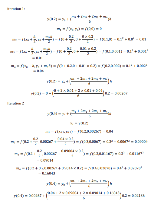
Example :

Use the classical RK method to estimate y(0.4) when 𝑦 ′ (𝑥) = 𝑥 ² + 𝑦 ² with 𝑦(0) = 0, assume h=0.2.

Solution
Given condition
𝑦(0) = 0, 𝑓(𝑥, 𝑦) = 𝑥 ² + 𝑦 ²

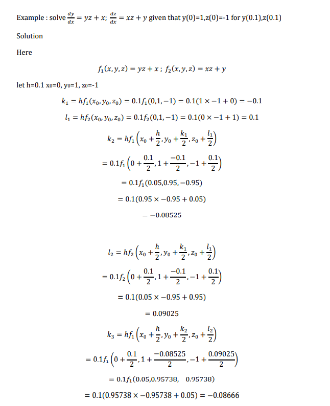
Runge Kutta method for simultaneous first order equation

Consider the simultaneous equation

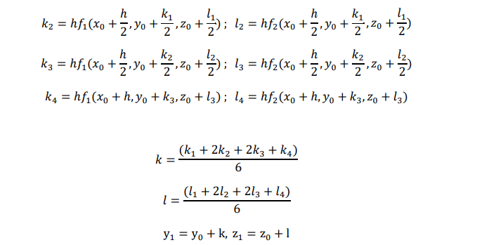
With the initial conditions 𝑦(𝑥₀) = 𝑦₀, 𝑧(𝑥₀) = 𝑧₀ now starting from (𝑥₀, 𝑦₀, 𝑧₀) the increment k and l in y and z are given by the following formula

𝑘₁ = ℎ𝑓₁(𝑥₀, 𝑦₀, 𝑧0) ; 𝑙₁ = ℎ𝑓₂(𝑥₀, 𝑦₀, 𝑧₀)

To compute y₂,z₂ we simply replace x₀,y₀,z₀ by x₁,y₁,z₁ in the above formulae

If we consider the second order R.K method

𝑘₁ = ℎ𝑓₁(𝑥₀, 𝑦₀, 𝑧₀) ; 𝑙₁ = ℎ𝑓₂(𝑥₀, 𝑦₀, 𝑧₀)

𝑘₂ = ℎ𝑓₁(𝑥₀ + ℎ, 𝑦₀ + 𝑘₁, 𝑧₀ + 𝑙₁) ; 𝑙₂ = ℎ𝑓₂(𝑥₀ + ℎ, 𝑦₀ + 𝑘₁, 𝑧₀ + 𝑙₁)

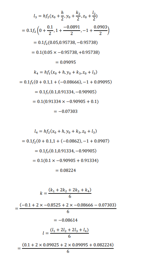
= 0.09077

𝑦₁ = 𝑦(0.1) = 𝑦₀ + 𝑘 = 1 + (−0.08614) = 0.91386

𝑧₁ = 𝑧(0.1) = 𝑧₀ + 𝑙 = −1 + 0.09077 = −0.90923

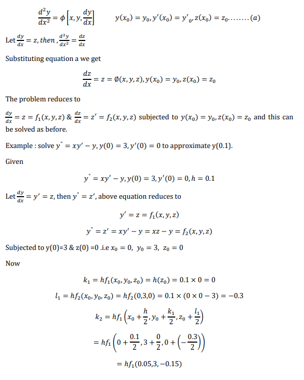
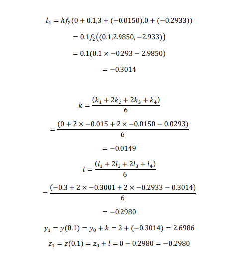
Higher order equation

A higher order differential equation is in the form

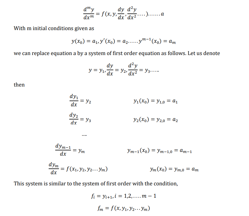
RK method for second order differential equations

Consider the second order differential equation

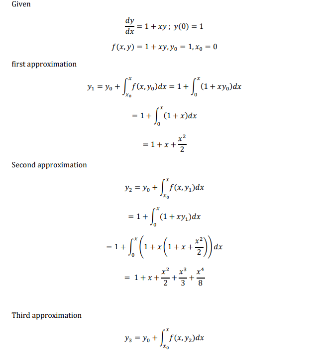
Picard method of successive approximation

Consider the first order differential equation 𝑑𝑦/ 𝑑𝑥 = 𝑓(𝑥, 𝑦) subjected to 𝑦(𝑥₀) = 𝑦₀. We can integrate this to obtain the solution in the interval(x₀,x).

The above equation can be written as dy = f(x, y)dx Integrating between the limits , we get

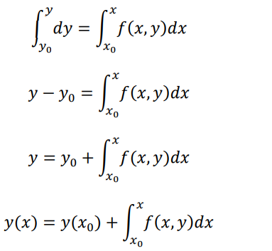
Since y appears under the integral sign on the right, the integration cannot be formed. The dependent variable should be replaced by either a constant or a function of x, since we know the initial value of y at x=x₀ we may use this as a first approximation to the solution and the result can be used on the right hand side to obtain the next approximation.

Now by Picard’s methods first approximation we replace y by y₀ in f(x,y) i.e

For second approximation y₂ replace y by y₁

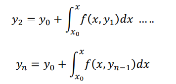
The process is to be stopped when two values of y, are same to desired degree of accuracy
Note:

• This method is applicable only to a limited class of equations in which the successive
  integration can be perform easily.
• Sometimes it may not be possible to carry out the integration.
• It is not convenient method for computer-based solution.

Example : Use Picard’s method to approximate the value of y when x=0.1,0.2,0.3,0.4 & 0.5.
given that y=1 at x=0, y’=1+xy, correct up to three decimal places

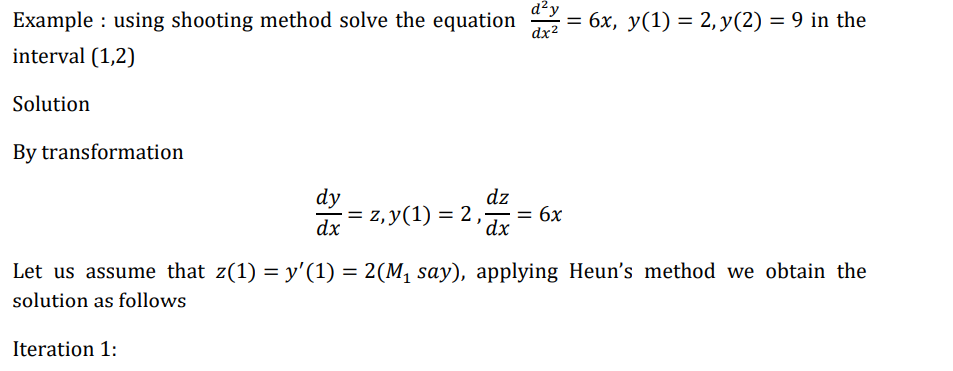
Shooting method

This method is called shooting method because it resembles an artillery problem. In this
method the given boundary value problem is first converted into an equivalent initial value
problem an then solved using any of the method discussed in previous section.
Consider the equation

𝑦 ” = 𝑓(𝑥, 𝑦, 𝑦 ′ ) 𝑦(𝑎) = 𝐴, 𝑦(𝑏) = B

Letting 𝑦 ′ = 𝑧, we obtain the following set of two equations 𝑦 ′ = 𝑧 , 𝑧 ′ = 𝑓(𝑥, 𝑦, 𝑧). In order to solve this set as initial value problem we need two conditions at x=a, we have one condition y(a)=A and therefore require another condtion for z at x=a. let us assume that 𝑧(𝑎) = 𝑀₁, where M₁ is a guess. Note M₁ represents the slope 𝑦 ′ (𝑥) 𝑎𝑡 𝑥 = 𝑎 thus the problem is reduced to as system two first order equation with initial conditions

𝑦 ′ = 𝑧𝑦(𝑎) = 𝐴

𝑧 ′ = 𝑓(𝑥, 𝑦, 𝑧)𝑧(𝑎) = 𝑀₁ … … (𝑎)

Equation a can be solved for y and z using any one step ,method suing steps of h, until the solution at x=b is reached. Let the estimated value of y(x) at x=b be B₁, if B₁=B then we have obtained the required solution. In practice it is very unlikely that our initial guess z(a)=M₁ is correct.

If 𝐵₁ ≠ 𝐵 then we obtain the solution with another guess say z(a) =M₂. Let new estimate of y(x) be at x=b be B₂. If B₂ is not equal to B then process is continued till we obtain the correct estimate of y(b). however the procedure can be accelerated by suing an improves guess for z(0) after estimates of B₁ & B₂ are obtained.

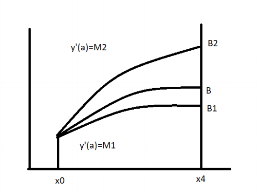
Let us assume that z(a)=M₃ lead to the value of y(b)=B, if we assume that values of M and B are linearly related then

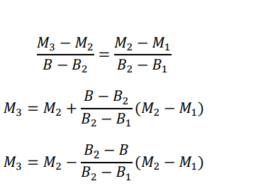
Now with z(a)=M₃, we can again obtain the solution of y(x).