Solution of Partial Differential, Elliptical, Parabolic, Hyperbolic Equations and their relevant examples

Many physical phenomena in applied science and engineering when formulated into
mathematical models fall into a category of system known as partial differential equations. A
partial differential equation is a differential equation involving more than one in independent
variables.
We can write a second order equation involving two independent variables in general form as :

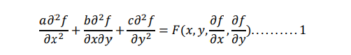
Where a,b,c may be constant or function of x & y

 The equation 1 is classified as

 i. Elliptical if 𝑏 ² − 4𝑎𝑐 < 0

ii. Parabolic if 𝑏 ² − 4𝑎𝑐 = 0

iii. Hyperbolic if 𝑏 ² − 4𝑎𝑐 > 0

Two approaches of solving are

1. Finite difference method (where regions are regular)
2. Finite element method (where regions are irregular)

Finite difference method

The finite difference method is based on the formula for approximating first and second order
derivatives of a function. In this method derivatives that occurs in partial differential equation are
replaced by their finite difference equivalents. The difference equation is then written for each
grid points using function values at the surrounding grid points. Solving these equations
simultaneously give the values of the function of each grid points.

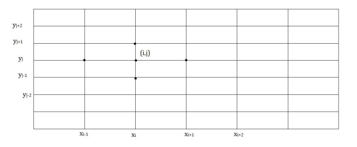
𝑥_𝑖+1 = 𝑥_𝑖 + ℎ

 𝑦_𝑖+1 = 𝑦_𝑖 + ℎ

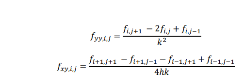
We have already discussed that if the function f(x) has a continuous fourth derivative, then it’s
first and second derivatives are given by the following central difference approximation.

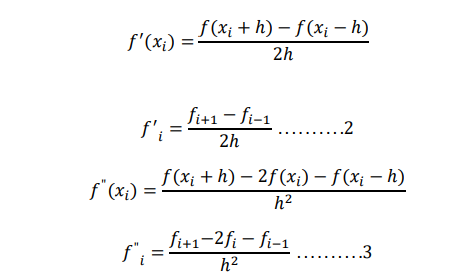
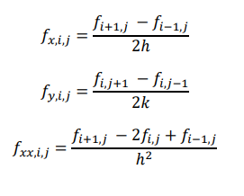
The subscripts on f indicate the x value at which the function is evaluated. When f is a function of
two variables x and y, the partial derivatives of f with respect x or y are the ordinary derivatives
of f with respect to x or y when y or x does not change. We can use the equations 2 and 3 in the x
direction to determine derivatives with respect to x and in the y direction to determine
derivatives with respect to y. thus we have

It would be convenient to use double subscripts i,j on f to indicate x and y values.

Then above equation becomes;

We will use these finite difference equivalents of the partial derivatives to construct various types
of differential equations.

Elliptical equations

Elliptical equations are governed by condition on the boundary of closed domain. We consider
here the two most commonly encountered elliptical equations.
a. Laplace’s equation
b. Poisson’s equation

Laplace’s equation

Any equation of the form ∇ ²𝑓 = 0 is called laplace’s equation, where

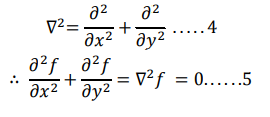
Where a=1,b=0,c=1 and F(x,y,𝜕𝑓 /𝜕𝑥 , 𝜕𝑓 /𝜕𝑦)=0

Where ∇ ² is called Laplacian operator, above equation can be written as

𝑈_𝑥𝑥 + 𝑈_𝑦𝑦 = 0

Replacing the second order derivatives by their finite difference equivalents, at points (𝑥_𝑖 , 𝑦_𝑖 ) we get

If we assume for simplicity, h=k, then we get

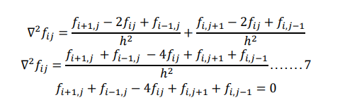
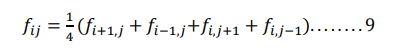
This is called Laplace’s equation Above equation contains four neighboring points around central points (𝑥_𝑖 , 𝑦_𝑖 ) as shown in figure, the above equation is known as five point difference formula for Laplace’s equation.

we can also represent the relationship of pivotal values pictorially as below.

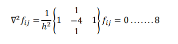
From above equation we can show that the function value at grid point(𝑥_𝑖 , 𝑦_𝑖 ) is the average of the values at the four adjoining points. i.e

To evaluate numerically the solution of Laplace equation at the grid points we can apply equation 9 at the grid points where 𝑓_𝑖𝑗is required thus obtaining a system of linear equations in the pivotal values of 𝑓_𝑖𝑗. The system of linear equations may be solved using either direct or iterative methods.

Example: Consider a steel plate of size 15cm x 15cm, if two of the side are held at 100^oc and other two side are held at 0^oc, what are the steady state temperature at interior points assuming a grid of 5cm x 5cm. Note: a problem with values known on each boundary is said to have Dirichlet boundary condition. This problem is illustrated below.

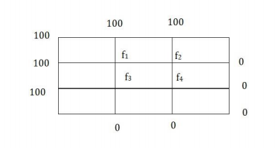
The system of equation is as follows

 Point 1:

100 + 100 + 𝑓₃ + 𝑓₂ − 4𝑓₁ = 0 … … . .1

Point 2:

𝑓₁ + 100 + 𝑓₄ + 0 − 4𝑓₂ = 0. . . . . . . .2

 Point 3:

100 + 𝑓₁ + 0 + 𝑓₄ − 4𝑓₃ = 0. . . . . . . .3

Point 4:

𝑓₃ + 𝑓₂ + 0 + 0 − 4𝑓₄ = 0. . . . . . . .4

 On solving above four equations we get the values as:

𝑓₁ = 75, 𝑓₂ = 50, 𝑓₃ = 50, 𝑓₄ = 25

So we can see the interior temperature points as above.

Poisson’s equation

If we put a=1, b=0, c=1 in the equation and F(x,y,f,𝑓_𝑥, 𝑓_𝑦)=g(x,y) then

The above equation a is called poisson’s equation using the notation 𝑔_𝑖𝑗 = 𝑔(𝑥_𝑖 , 𝑦_𝑖) and laplace equation may be modified to solve the equation a. the finite difference formula for solving poisson’s equation then takes of the form

Example: Solve the poisson’s equation ∇ ²𝑓 = 2𝑥 ²𝑦 ² over the square domain 0 ≤ 𝑥 ≤ 3 & 0 ≤ 𝑦 ≤ 3 with f=0 on the boundary and h=1.

The domain is divided into squares of one unit size as in figure.

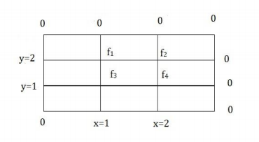
By applying equations b at each grid points

 Point 1:

 0 + 0 + 𝑓₃ + 𝑓₂ − 4𝑓₁ = 1 ²𝑔(1,2)

𝑓₂+𝑓₃ − 4𝑓₁ = 2𝑥₁ 2𝑥2²

 𝑓₂+𝑓₃ − 4𝑓₁ = 8 . . . . . . . . 1

Point 2:

 𝑓₁ + 0 + 0 + 𝑓₄ − 4𝑓₂ = 1

 2𝑔(2,2) 𝑓₁+𝑓₄ − 4𝑓₂ = 2𝑥2 ²𝑥2 ²

𝑓₁ − 4𝑓₂ + 𝑓₄ = 32 . . . . . . . . 2

Point 3:

 0 + 𝑓₁ + 0 + 𝑓₄ − 4𝑓₃ = 1 ²𝑔(1,1)

 𝑓₁+𝑓₄ − 4𝑓₃ = 2𝑥1 ²𝑥1 ²

𝑓₁ − 4𝑓₃ + 𝑓₄ = 2 . . . . . . . . 3

 Point 4:

𝑓₃ + 𝑓₂ + 0 + 0 − 4𝑓₄ = 1 ²𝑔(2,1)

𝑓₂+𝑓₃ − 4𝑓₄ = 2𝑥2 ² 𝑓₂ + 𝑓₃ − 4𝑓₄ = 8 . . . . . . . . 4

On solving we get

Therefore the interior points are as above.
Note: we can use any problem-solving methods already discussed for solving the values of fi

Parabolic equations

Elliptical equations studies previously described problems that are time independent, such problems are known as steady state problems, but we come across problems that are not steady state. This means that the function is dependent on both space and time. Parabolic equations for which 𝑏 ² − 4𝑎𝑐 = 0, describes the problem that depend on space and time variables.

A popular case for parabolic type of equation is the study of heat flow in one-dimensional direction in an insulated rod, such problems are governed by both boundary and initial conditions.

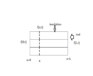
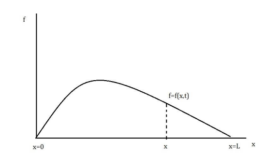
Let f represent the temperature at any points in rod, whose distance from left end is x. Heat is
flowing from left to right under the influence of temperature gradient. The temperature f(x,t) in
the at position x and time t governed by the heat equation.

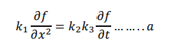
Where 𝑘₁is coefficient of thermal conductivity, 𝑘₂ is the specific heat and 𝑘₃ is density of the material.

Equation a can be simplified as

𝑘𝑓_𝑥𝑥(𝑥,𝑡) = 𝑓_𝑡 (𝑥,𝑡) … … . b

Where 𝑘 = 𝑘1/ 𝑘2𝑘

The initial condition will be the initial temperatures at all points along the rod .
𝑓(𝑥, 0) = 𝑓(𝑥) 0 ≤ 𝑥 ≤ 𝐿

The boundary conditions f(0,t) and f(L,t) describes the temperature at each end of the rod as
function of time, if they are held at constant then
𝑓(0,𝑡) = 𝑐10 ≤ 𝑡 ≤ ∞
𝑓(𝐿,𝑡) = 𝑐2 0 ≤ 𝑡 ≤ ∞

solution of heat equation
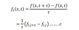
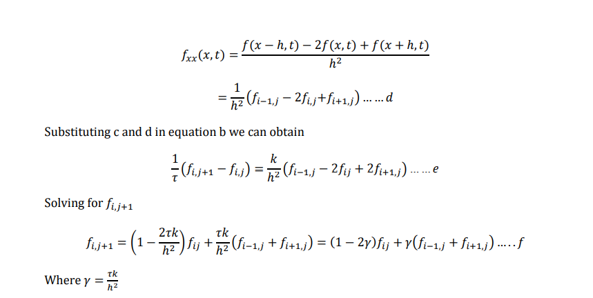
we can solve the heat equation in equation using the finite difference formula given below.

Bender Schmidt method

he recurrence of equation allows us to evaluate f at each point x and at any point t. if we choose
step size ∆𝑡 & ∆𝑥, such that

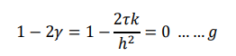
Equation f simplifies to

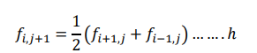
Equation h is known as Bender Schmidt recurrence equation. This equation determines the value of f at 𝑥 = 𝑥_𝑖 , at time 𝑡 = 𝑡_𝑖 + 𝜏 as the average of the values right and left of 𝑥_𝑖 at time 𝑡_𝑗.

Note that the step size in ∆𝑡 obtained from equation g.

𝜏 = ℎ ² / 2𝑘

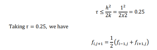
Gives the equation h , equation f is stable if and only if the we step size 𝜏 satisfies the condition

𝜏 ≤ ℎ ² / 2k

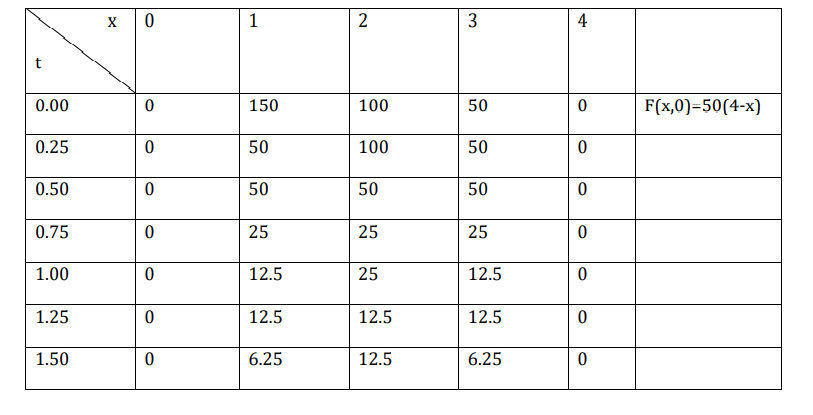
Example : Solve the equation 2𝑓_𝑥𝑥(𝑥,𝑡) = 𝑓_𝑡(𝑥,𝑡) , 0 < 𝑡 < 1.5 𝑎𝑛𝑑 0 < 𝑥 < 4 given the initial condition

𝑓(𝑥, 0) = 50(4 − 𝑥)0 ≤ 𝑥 ≤ 4
And boundary condition
𝑓(0,𝑡) = 0, 0 ≤ 𝑡 ≤ 1.5
𝑓(4,𝑡) = 0, 0 ≤ 𝑡 ≤ 1.5
Solution
If we assume ∆𝑥 = ℎ = 1, ∆𝑡 = 𝜏 (using Bender Schmidt method)

Using the formula we can generate successfully f(x,t). the estimated are recorded in the following
table at each interior point, the temperature at any single point is just average of the values at the
adjacent points of the previous points.

Hyperbolic equation

Hyperbolic equation models the vibration of structure such as building beams and machines we
here consider the case of a vibrating string that is fixed at both the ends as figure.

The lateral displacement of string f varies with time t and distance x along the string. The
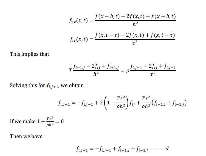
displacement f(x,t) is governed by the wave equation

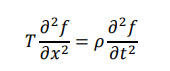
Where T is the tension in the string and ρ is the mass per unit length.
Hyperbolic problems are governed by both boundary and initial conditions, if time is one of the
independent variables. Two boundary conditions are the vibrating string problems under
consideration are
𝑓(0,𝑡) = 0, 0 ≤ 𝑡 ≤ 𝑏
𝑓(𝐿,𝑡) = 0, 0 ≤ 𝑡 ≤ 𝑏
Two initial condition are
𝑓(𝑥, 0) = 𝑓(𝑥), 0 ≤ 𝑡 ≤ 𝛼
𝑓_t(𝑥, 0) = 𝑔(𝑥), 0 ≤ 𝑡 ≤ 𝑎

Solution hyperbolic equations
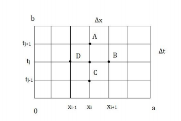
The domain of interest 0 ≤ 𝑡 ≤ 𝑎 𝑎𝑛𝑑 0 ≤ 𝑡 ≤ 𝑏 is partitioned as shown in figure, the rectangle
size is ∆𝑥 = ℎ, ∆𝑡 = 𝜏

The difference equation for 𝑓_𝑥𝑥(𝑥,𝑡) 𝑎𝑛𝑑 𝑓_𝑡𝑡(𝑥,𝑡) are

The values of f at 𝑥 = 𝑥_𝑖 and 𝑡 = 𝑡_𝑗 + 𝜏 is equal to the um of the values of f, at the point 𝑥 = 𝑥_𝑖 − ℎ and 𝑥 = 𝑥_𝑖 + ℎ at the time 𝑡 = 𝑡_𝑗 (𝑝𝑟𝑒𝑣𝑖𝑜𝑢𝑠 𝑡𝑖𝑚𝑒) minus the value of f at 𝑥 = 𝑥_𝑖at time 𝑡 = 𝑡_𝑗 − 𝜏.

From figure we can say

𝑓_𝐴 = 𝑓_𝐵 + 𝑓_𝐷 − 𝑓_C

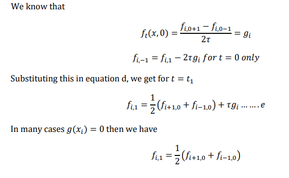
Starting values
We need two rows of starting values, corresponding to j=1 and j=2, in order to computer the
values of the third row. First row is obtained using the condition.
𝑓(𝑥, 0) = 𝑓(𝑥)

The 2^nd row can be obtained using the 2^nd initial condition as 𝑓_𝑡 (𝑥, 0) = 𝑔(𝑥)

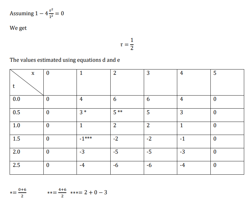
Example: Solve numerically the wave equation

𝑓_𝑡𝑡(𝑥,𝑡) = 4𝑓_𝑥𝑥(𝑥,𝑡)0 ≤ 𝑥 ≤ 5 & 0 ≤ 𝑡 ≤ 2.5

With boundary condition

𝑓(0,𝑡) = 0 𝑎𝑛𝑑𝑓(5,𝑡) = 0

And initial values

 𝑓(𝑥, 0) = 𝑓(𝑥) = 𝑥(5 − 𝑥)

𝑓_𝑡 (𝑥, 0) = 𝑔(𝑥) = 0

Solution
Let h=1
Given 𝑇/𝜌 = 4

Reference 1 : Numerical Methods , Dr. V.N. Vedamurthy & Dr. N. Ch. S. N. Iyengar, Vikas Publishing House.